DOI:10.28974/idojaras.2018.4.6
IDŐJÁRÁS
Quarterly Journal of the Hungarian Meteorological Service Vol. 122, No. 4, October – December, 2018, pp. 453–462
Methodology of objective three-dimensional identification and tracking of cyclones and anticyclones in the low and
middle troposphere
Evhen V. Samchuk
Ukrainian Hydrometeorological Institute Nauky av., 37, 03028 Kyiv, Ukraine Authors E-mail: evhen.samchuk@gmail.com (Manuscript received in final form October 25, 2017)
Abstract — Extratropical cyclones and anticyclones are the main objects in researches of the large-scale atmospheric circulation processes in midlatitudes. In this context, new data which can improve our knowledge about their typical places of origin, tracks, and lifetime characteristics were critical.
The purpose of this research is to analyze existing methods and algorithms, used for cyclone and anticyclone identification and tracking, and to develop a three-stage methodology of baric systems identification in the low and middle troposphere based on a three-dimensional approach.
This research utilizes 40-year-long datasets of sea level pressure and geopotential height of three standard pressure levels up to 500 hPa covering the Northern hemisphere down to 20°N.
This paper presents a newly developed unified baric systems identification and tracking methodology. It is based on a step-by-step identification of isolated clusters of low and high sea level pressure and geopotential height throughout the low and middle troposphere from the ground level to 500 hPa pressure level. Centers of clusters on different levels for each moment of time are combined in a single vertical profile which represents one certain baric system. Tracking of the baric system movement is realized with nearest neighbor method, improved for more accurate detection and tracking of fast- moving short-living cyclones. In the process, a software was developed for the purposes of the automatic identification of baric systems in the Northern Hemisphere and for creating sets of cinematic schemes of natural synoptic periods. Also, a database of the baric systems existed during on the period of 1976–2015 on the Northern Hemisphere was created.
Key-words: objective identification, baric system, cyclone, anticyclone, reanalysis, trajectories, software.
1. Introduction
Among all processes occurring in the atmosphere, cyclonic and anticyclonic activities are the most fundamental and persistent. It includes formation, evolution, movement and decline of cyclones and anticyclones in the lower and middle troposphere in the midlatitudes of the Northern Hemisphere. This process provides transportation and distribution of atmospheric energy, heat, and moisture on the global scale, so objective knowledge of its progress is vital for description and systematization of the different weather regimes. The best way of this systematizaion in the traditions of the soviet synoptic school, which is still represented at the Ukrainian weather service, is a compiling of the so-called 'joint kinematic maps' of the natural synoptic periods. Despite of the critical importance of such activities in understanding of the state of the atmosphere and its tendencies, it is still fully performed in manned mode without any automation.
On the one hand, identification and tracking of extratropical cyclones is heavily studied due to their significant role in a wide spectrum of weather phenomena. Thus, there is no surprise that in the last 20 years numerous different methods of cyclone identification and tracking were developed and applied (Alpert et al., 1990; Murray and Simmonds, 1991; Keonig et al., 1993;
Hodges, 1994; Serreze, 1995; Sinclair, 1997; Sickmoller et al., 2000; Klawa and Ulbrich, 2003; Hanson et al., 2004; Bengtsson et al., 2006; Wernli and Schwierz, 2006; Raible et al., 2008; Inatsu, 2009). Each of them is based on different perceptions of what cyclone is, and utilizes different atmospheric variables, such as sea level pressure (Benestad and Chen, 2006), its gradient (Leckebusch et al., 2006), geopotential height of 1000 (Blender and Schuber, 2000) and 850 hPa (Hewson and Titley, 2010) pressure levels, Laplasian of the geopotential height (Balabukh, 2005; Neu U. et al., 2010; Trigo, 2011) and potential vorticity (Kew et al., 2010). Each of these methods has its limitations, determining conditions under which localized baric system could be ignored, such as distance of day-to-day displacement, duration of existence, or elevation above sea level of the region of baric system existence (Pinto et al., 2005). On the other hand, results provided by these methods are hard to intercompare.
Also, the most frequently used variable in these methods is a sea level pressure, while higher levels of troposphere are ignored. Besides, a very few information about anticyclone identification and tracking methods can be found due to their less dangerous overall impact on weather.
Taking all into account the above mentioned facts, the necessity of a reliable and universal methodology of three-dimensional identification of both cyclone and anticyclone became clear.
The full-scale methodology of the three-dimensional baric systems identification consists of three stages:
1. Localization of the low and high pressure centers in the sea level pressure (SLP) fields and on the pressure surfaces (850, 700, and 500 hPa).
2. Combination of the centers into a vertical profile of a single baric system.
3. Tracking of baric system movement and evolution during its whole lifecycle.
2. Initial data and methods
This research utilizes the 40-year-long NCEP/NCAR Reanalysis dataset, including 4-time daily sea level pressure (SLP) fields, and the geopotential height of the 850, 700, and 500 hPa pressure surfaces (ESRL: PSD:
NCEP/NCAR Reanalisys 1). The period of interest is from 1976 to 2015, and the research region includes part of the Northern Hemisphere from 20°N to the north. All algorithms are realized with C# programming language under .NET platform using Windows Forms technology. GDI+ programming interface was used for maps composition and graphics visualization.
3. Localization of the pressure centers
Fig. 1 shows a part of the region of interest and also represents every grid node within it. It is important to emphasize that each square on the map represents one single node of a grid, which means that the node’s actual position is referred to as the center of a square. Numbers near the x and y axis refers to the numbers of grid columns and rows inside the original dataset correspondently. Every number (N) can be translated into latitude or longitude using Eqs. (1) and (2):
90
5 .
2 +
−
= N
ϕ . (1)
N 5 .
= 2
λ . (2)
Also it is necessary to explain such a large region of interest in this research. While other identification methods has been tested on relatively small regions, such as Europe or the North Pacific region, in this case the Northern Hemisphere was chosen in order to avoid unnecessary accuracy drops even in face of the bigger amount of data to analyze and time to spend. The reason of this choice is inside of the form the logical representation of initial data. Dataset transfer data are derived from the Earth's spherical surface into a two- dimensional array, each cell of which represent a single node of a grid.
In case of an array, which covers the whole Northern Hemisphere, the left side of this rectangle is actually a continuation of the right one. But in the logic model there are two opposite sides of the region of interest, so any analysis of the geometric shape of the SLP or the geopotential field, performed on limited area without taking this data feature into account, leads to a critical failure on both left and right edges.
The method of center’s localization, described below, does take this feature into account, so on one hand it is protected from erroneous detection, and on the other
hand it covers entire hemisphere, allowing further study of atmospheric circulation in any region on demand.
Fig. 1. Stages of grid nodes filtering during the localization of the pressure centers.
The first stage is accomplished through the method of regular grid nodes filtering. Employment of this method will be demonstrated on the localization of low-pressure centers in the SLP field. All statements are applicable to the localization of the rest types of centers with few clauses, which will be mentioned later.
Localization of a low-pressure center in the SLP field is performed through the allocation of isolated low-pressure clusters via regular grid nodes iterative filtering. The first step is calculating of pressure minima within the grid, which hereinafter will be a reference value. Then this value is replace with the nearest number that is greater than it and is a multiple of 5 (according to the rules of hemisphere-scale SLP charts composing isobar values which are always a multiple of 5). Then, among all nodes of grid, only that ones are picked into the initial array for analysis, in which the pressure is less than reference value (Fig. 1a, light gray squares). At this stage of progress, nodes, contained in the initial array are divided into separate clusters. Each cluster contains nodes that directly adjoin each other and does not adjoin nodes from any other clusters. As it can be seen from Fig. 1a, initial array was divided into two separate clusters – one in the polar region and the other one, which contains only one grid node, near Greenland.
For each of these clusters, the node with the local minima of pressure and the node, representing the geometrical center of the cluster, are designated. Grid node of a cluster with coordinates (φg, λg) which satisfies condition (Eq.(3)) is marked as the geometrical center of the cluster:
min
1
2
2
( )
)
(
+ = − −
= n
i
ϕ
gϕ
iλ
gλ
i . (3)For now, only the deepest centers of the grid are picked up, so the reference value is incremented by 5 hPa, and the clusterization procedure repeats. Thus, beginning from the second procedure iteration, additional node filtering are involved. Because of the repetitive picking of the previously analyzed nodes, fresh-composed clusters will consist of grid nodes, which werre already used on the previous iteration or directly adjoin them. (Fig. 1b, dark gray squares). To avoid this, all nodes, adjoining previously composed clusters, are ignored and only previously uncharted centers are brought to the analysis (Fig. 1c, dark gray squares). Applying this additional filtering allows to decrease the time expenses by 5 times, which is vital in case of lack of computing resources and large time periods to process. As a result, the analysis of a single field takes nearly 1 second even on low-end computers, independently from the field structure and the seasons of the year. The described clusterization procedure is repeated until the reference value is lower than 1020 hPa, which is the boundary between cyclonic and anticyclonic fields.
The identification procedure has a few features while applying in different conditions. Thus, when localizing high-pressure centers in the SLP field, firstly the grid pressure maxima is picked up as reference value, and then it is iteratively decreased to 1020 hPa. On the pressure surfaces, the reference value decreases and increases by 4 geopotential decameters. Besides, there is no field division into cyclonic and anticyclone parts, and both high- and low-pressure centers localized through all available reference values from grid minima to maxima.
Results of the center localization on each level are stored in the database, which contains information about every localized center, such as its type (low- or high-pressure), pressure level, where center has been localized, coordinates of grid node with extreme pressure value within every unique cluster, as well as coordinates of its geometrical center.
There is a reason why the terms ‘cyclone’ and ‘anticyclone’ were avoided previously. Centers, localized on the first stage of the baric system identification, cannot be directly associated with a particular cyclone or anticyclone, because these centers are only the grid nodes, outlined with isoline. Thus, the question of belonging of each center to the real baric system remains uncertain on this stage.
This uncertainty resolves on the next stage of the baric systems’ identification, where the composition of their vertical profile is taking place.
4. Composing of the baric system profile
Vertical profile is a source of valuable characteristics of the baric system. First of all, it describes its vertical extension, which allow us to assign the examined system to one of the principal groups: low, middle, high, or upper baric system.
Also, the profile's tilt angle is specific for each stage of the baric system lifetime.
Profile of a new-formed baric system has significant slant on the higher levels, but on the later stages it is negligible. Last, but not least: composing a vertical profile allows us to operate with such terms as ‘cyclone’ and ‘anticyclone’, which were avoided earlier, and to treat identified structures as full-scale baric systems, which exists not only on one particular level, but in a whole thickness of the low and middle troposphere.
Algorithm of the baric system profile composition uses characteristics of the previously localized centers as raw data. The geometrical location of the center, localized in the SLP field, became the first point of the profile. After that, the algorithm searches for centers suitable for the current profile, on each of the rest levels. The only condition of including a center into profile is localization of one within a radius of 500 km from the previous profile point. After that the centers selected by the profile completion are removed from the initial array, the procedure is repeated until all centers are involved in profiles, independently from the level where profile composition begins. The result of this procedure is an array of the profile entities. Each profile entity contains detailed
characteristics of each profile point as well as generic characteristics of each profile, such as type, number of involved levels, and averaged geographical coordinates of profile which represent the general position of a baric system in the atmosphere. Also, all profiles which involve only one level are removed from the result collection.
5. Baric system tracking
The final stage of the baric system identification implies the nearest neighbor method also known as NN-method (Fix and Hodges, 1951) for cyclones and anticyclones tracking, using baric systems coordinates obtained on the previous stage. From this point, coordinates of each baric system will be mentioned as
‘nodes’. By this approach, every node can be included into a trajectory when its distance from the previous and next trajectory nodes is minimal. The maximum distance between trajectory nodes is limited to 700 km. This distance corresponds to a baric system movement speed of 110 km/h, which surely exceeds the actual velocities of fast-moving cyclones, preventing trajectory division. Analysis of manually composed cyclone and anticyclone tracks showed that in nearly 35% of cases, the opposite issue takes place when two cyclones tracks are composed into a single one when one of them declines nearby another. Low time resolution (12 hours and more) of initial data promotes this issue as well. This is the reason why the nearest neighbor method was improved with one significant modification to prevent such issues.
Beginning from the second node of any trajectory, additional movement direction verification is applied to prevent combining two different cyclones into one trajectory. This verification checks directions of the cyclone movement on two adjacent sections of the trajectory. If movement directions on these sections are opposite or directed closely opposite one to another, the last node is not included into the trajectory, but trajectory compositions are continued. The distance limit increases by 1.5 times, and the next node of trajectory is picked up among centers of the next time stamp. If the algorithm is unable to find the next trajectory node under this condition, the trajectory composition interrupts completely, and the distance limit returns to the original value. Also, all trajectories that last for less than 24 hours are ignored. Similarly to the first two stages of the baric system identification, results of trajectory composition are stored in the database.
6. Accuracy assessment
Objective assessment of the accuracy of the described methodology is obviously complicated, because each stage itself also demands accuracy assessment. Due to lack of similar researches, dedicated to the same period and region, accuracy
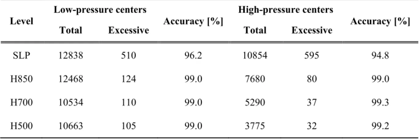
assessment was performed through visual control of correspondence between the location of identified centers on each pressure level and its actual location on the map. The comparison covers the whole year of 2015 and involves almost six thousands unique maps of SLP (4 maps per day) and geopotential height on three pressure levels (12 maps per day). This verification has demonstrated a weak spot of the localization algorithm associated with the features of input data. In cases, when gridded data contain single nodes which can be outlined with isolines, excessive center localization takes place. It is caused by the incapability of displaying nodes with grid translation into conical projection during the map composition. However, it decreases the accuracy of center localization only by 5% in the SLP field and less than 1% on the rest of the pressure levels (Table 1). Nevertheless, it can not affect the accuracy of the baric system identification, because such erroneously localized centers will not be included into the vertical profile.
Table 1. Accuracy of the localization of high- and low-pressure centers on each level
Level
Low-pressure centers
Accuracy [%]
High-pressure centers
Accuracy [%]
Total Excessive Total Excessive
SLP 12838 510 96.2 10854 595 94.8
H850 12468 124 99.0 7680 80 99.0
H700 10534 110 99.0 5290 37 99.3
H500 10663 105 99.0 3775 32 99.2
Due to modifications applied to the NN-method, tracking efficiency has been significantly improved, especially in cases of several intensive, fast- moving cyclones, which develop and decline nearby to each others. The increased criteria, applied to anticyclone tracking, prevent fragmentation of long-living stationary anticyclone trajectory caused by center displacement. The iscovered issues affect only the first stage of the entire procedure and can be ignored. Thus, overall climatology of both cyclone and anticyclone activities sustain minimal impact.
7. Conclusions
The developed methodology reflects new perspective on the baric system identification and tracking with classic synoptic perception of cyclones and anticyclones as three-dimensional structures, covering few vertical levels at once. This approach appears in a multi-staged algorithm, which provides relievable data about the lifetime characteristics of cyclones and anticyclones.
The reliability of the results is provided through objective limitations, derived from issues, found during analysis of manually performed identification procedure. The assessment of the new identification methodology’s accuracy showed it extremely high precision compared to the manual identification. Also, algorithm optimization tends to decrease the time expense, allowing running identification procedure on big time periods without any necessity for a powerful computer. The developed database (with generic and detailed characteristics of the cyclones and anticyclones, which existed in the Northern Hemisphere in the period of 1976–2015) can be used for the further study of any kind of specific types of the large-scale atmospheric processes, such as atmospheric blocking, southern cyclones, etc.
References
Alpert P., Neeman B.U., and Shay-El Y., 1990: Climatological analysis of Mediterranean cyclones using ECMWF data. Tellus 42A, 65–77.
Balabukh V., 2005: Objective identification of synoptic-scale baric systems. Taras Shevchenko Nat.
Univ. Kyiv Bull. 51, 49–50.
Benestad, RE. and Chen, D., 2006: The use of a calculus-based cyclone identification method for generating storm statistics. Tellus 58A, 473–486.
https://doi.org/10.1111/j.1600-0870.2006.00191.x
Bengtsson, L.K., Hodges K.I., and Roeckner, E., 2006: Storm tracks and climate change. J.Climate 19, 3518–3543. https://doi.org/10.1175/JCLI3815.1
Blender, R. and Schubert, M., 2000: Cyclone tracking indifferent spatial and temporal resolutions.
Month. Weather Rev. 128, 377–384.
https://doi.org/10.1175/1520-0493(2000)128<0377:CTIDSA>2.0.CO;2 ESRL: PSD: NCEP/NCAR Reanalisys 1:
https://www.esrl.noaa.gov/psd/data/gridded/data.ncep.reanalysis.html
Fix E. and Hodges, J.L., 1951: Discriminatory analysis, nonparametric discrimination, consistency properties. U.S. Air Force School of Aviation Medicine, Randolf Field, Texas, Project 21-49- 004, Contract AF 41(128)-31, Rep. 4, 1951.
Hanson, C.E., Palutikof, J.P., and Davies, T.D., 2004: Objective cyclone climatologies of the North Atlantic – a comparision between ECMWF and NCEP reanalysis. Climate Dynam. 22, 757–769. https://doi.org/10.1007/s00382-004-0415-z
Hewson, T.D. and Titley H. A., 2010: Objective identification, typing and tracking of the complete life- cycles of cyclonic features at high spatial resolution. Meteorol. Appl. 17, 355–381.
https://doi.org/10.1002/met.204
Hodges, K.I., 1994: A general method for tracking analysis and its applications to meteorological data, Month. Weather Rev. 122, 2573–2586.
https://doi.org/10.1175/1520-0493(1994)122<2573:AGMFTA>2.0.CO;2
Inatsu, M., 2009: The neighbor enclosed area tracking algorithm for extratropical wintertime cyclones.
Atmos. Sci. Lett. 10, 267–272. https://doi.org/10.1002/asl.238
Kew, S.F., Sprenger, M., and Davies, H.C., 2010: Potential vorticity anomalies of the lower most stratosphere: A 10-yr winter climatology. Month. Weather Rev. 138, 1234–1249.
https://doi.org/10.1175/2009MWR3193.1
Keonig, W., Sausen, R., and Sielmann, F., 1993: Objective identification of cyclones in GCM simulations. J. Climate, 6, 2217–2231.
https://doi.org/10.1175/1520-0442(1993)006<2217:OIOCIG>2.0.CO;2
Klawa, M. and Ulbrich, U., 2003: A model for the estimation of storm losses and the identification of severe winter storms in Germany. Nat. Haz. Earth Syst. Sci. 3, 725–732.
https://doi.org/10.5194/nhess-3-725-2003
Leckebusch, G.C., Koffi, B., Ulbrich, U., Pinto, J.G., Span-Gehl, T., and Zacharias, S., 2006: Analysis of frequency and intensity of winter storm events in Europe on synoptic and regional scales from a multi-model perspective, at synoptic and regional scales. Climate Res. 31, 59–74.
https://doi.org/10.3354/cr031059
Murray, R.J. and Simmonds, I., 1991: A numerical scheme for tracking cyclone centres from digital data, part 1: development and operation of the scheme. Australian Meteorol. Mag. 39, 155–156.
Neu, U., Akperov, M.G.; Bellenbaum, N.; Benestad, R., Blender, R., Caballero, R., Cocozza, A., Dacre, H.F., Feng, Y., Fraedrich, K., Grieger, J., Gulev, S., Hanley, J., Hewson, T., Inatsu, M., Keay, K., Kew, S.F., Kindem, I., Leckebusch, G.C., Liberato, M.L.R., Lionello, P., Mokhov, I.I., Pinto, J.G., Raible, C.C., Reale, M., Rudeva, I., Schuster, M., Simmonds, I., Sinclair, M., Sprenger, M., Tilinina, N.D., Trigo, I.F., Ulbrich, S., Ulbrich, U., Wang, Xi.L., and Wernli, H., 2013: IMILAST: A Community Effort to Intercompare Extratropical Cyclone Detection and Tracking Algorithms. Amer. Meteorol. Soc. 94, 529–547.
https://doi.org/10.1175/BAMS-D-11-00154.1
Pinto, J.G., Spangehl, T., Ulbrich, U., and Speth, P., 2005: Sensitivities of a Cyclone Detection and Tracking Algorithm: Individual Tracks and Climatology. Meteorol. Zeitschrift 14, 823–838.
https://doi.org/10.1127/0941-2948/2005/0068
Raible, C., Della-Marta, P.M., Schewierz, C., Wernli, H., and Blender, R., 2008: Northern hemipshere extratropical cyclones: A comparison of detection and tracking methods and different reanalysis. Month. Weather Rev. 136, 880–897. https://doi.org/10.1175/2007MWR2143.1
Serreze, M.C., 1995: Climatological aspects of cyclone development and decay in the Arctic. Atmos.–
Ocean 33, 1–23. https://doi.org/10.1080/07055900.1995.9649522
Sickmoller, M., Blender, R., and Fraedrick, K., 2000: Observed winter cyclone tracks in the northern hemisphere in reanalysed ECMWF data. Quart. J. Roy. Meteorol. Soc. 126, 591–620.
https://doi.org/10.1002/qj.49712656311
Sinclair, M.R., 1997: Objective identification of cyclones and their circulation intensity and climatology. Weather Forecast. 12, 595–612.
https://doi.org/10.1175/1520-0434(1997)012<0595:OIOCAT>2.0.CO;2
Trigo, R. and Klaus, M., 2011: An exceptional winterstorm over northern Iberia and southern France.
Weather 66, 330–334. https://doi.org/10.1002/wea.755
Wernli H. and Schwierz C., 2006: Surface cyclones in the ERA-40 data set (1958–2001). Part 1: Novel identification method and global climatology. J. Atmos. Sci. 63, 2486–2507.
https://doi.org/10.1175/JAS3766.1