DOI:10.28974/idojaras.2018.2.2
IDŐJÁRÁS
Quarterly Journal of the Hungarian Meteorological Service Vol. 122, No. 2, April – June, 2018, pp. ?–?
Evaluation of ozone deposition models over a subalpine forest in Niwot Ridge, Colorado
Dalma Szinyei1, 2, Györgyi Gelybó*3, Alex B. Guenther4, Andrew A. Turnipseed5, Eszter Tóth3 and Peter J. H. Builtjes6,7
1 MTA-PE Air Chemistry Research Group, University of Pannonia, Egyetem u. 10, H-8200, Veszprém, Hungary
2 Department of Geology and Meteorology, University of Pécs, Ifjúság útja 6, H-7624, Pécs, Hungary
3 Institute for Soil Sciences and Agricultural Chemistry, Centre for Agricultural Research, Hungarian Academy of Sciences,
Herman Ottó út 15, H-1022, Budapest, Hungary
4Department of Earth System Science University of California, Irvine CA 92697, USA
5 Atmospheric Chemistry Division, National Center for Atmospheric Research, P.O. Box 3000, Boulder, CO 80307-3000, USA
6 TNO Built Environment and Geosciences, Air Quality and Climate Team, Princetonlaan 6, 3508 TA, Utrecht, The Netherlands
7 Institute of Meteorology, Freie Universität Berlin, Carl-Heinrich-Becker Weg 6-10, 12165, Berlin, Germany
*Corresponding author E-mail: gelybo.gyorgyi@agrar.mta.hu (Manuscript received in final form April 10, 2017)
Abstract⎯In this study, we evaluated three conceptually similar ozone gas deposition models. These dry deposition models are frequently used with chemical transport models for calculations over large spatial domains. However, large scale applications of surface- atmosphere exchange of reactive gases require modeling results as accurate as possible to avoid nonlinear accumulation of errors in the spatially representative results. In this paper, model evaluation and comparison against measured data over a coniferous forest at Niwot Ridge AmeriFlux site (Colorado, USA) is carried out. At this site, no previous model calibration took place for any of the models, therefore, we can test and compare their performances under similar conditions as they would perform in a spatial application. Our results show systematic model errors in all the three cases, model performance varies with time of the day, and the errors show a pronounced seasonal pattern as well. The introduction of soil moisture content stress in the model improved model performance regarding the magnitude of fluxes, but the correlation between measured and modeled ozone deposition values remains low. Our results suggest that ozone dry deposition model results should be interpreted carefully in large scale applications, where the accuracy can vary with land cover sometimes are biased.
Key-words: ozone fluxes, deposition model, big leaf models, coniferous forest
1. Introduction
Air quality monitoring and modeling is important not only to quantify the environmental stress on human health but also to understand the impact on terrestrial ecosystems. Many relevant studies, using field measurements and/or model results, have reported that tropospheric ozone can influence the health of the ecosystem (namely, Fares et al., 2013; Loreto and Fares, 2007). Ozone (O3) like some other trace gases passes through the stomata into the mesophyll cells of plants and is toxic since it reacts with the liquid components of the apoplast to create reactive oxygen species (Fares et al., 2013). These can oxidize the cell walls to start a cascade of reactions which lead, at the final stage, to cellular death (Fares et al., 2013). Karnosky et al. (2003; 2005) reported significant ecosystem scale responses to elevated carbon dioxide (CO2) and O3 levels in the Aspen FACE Experiment. The changes were reflected in several ecosystem properties, including photosynthesis. Their results suggest that elevated O3 at relatively low concentrations can significantly reduce the growth enhancement by elevated CO2.
As forests can be long-term sinks of carbon (Pan et al., 2011), they play a key role in terrestrial ecosystem-atmosphere interactions. Any productivity changes caused, e.g., by detrimental effects of the ozone can have serious effects on atmospheric CO2 concentrations as well (Ashmore, 2005; Klinberg et al., 2011). Anav et al. (2011) investigated the effects of tropospheric O3 on photosynthesis and leaf area index on European vegetation using a land surface model (ORCHIDEE) coupled with a chemistry transport model (CHIMERE).
Their results showed that the effect of ozoneon vegetation leads to a reduction in yearly gross primary productivity (GPP) of about 22% and a reduction in leaf area index (LAI) of 15–20%. Decrease in GPP probably becomes more acute due to the harmful effect of tropospheric ozone. Based on high methane level scenarios (RCP8.5, SRES A2) (Kirtman et al., 2013), it is predicted that background surface ozone will increase about 8ppb on average by 2100 (25% of current levels) relative to scenarios with small methane changes (RCP4.5, RCP6.0). Background tropospheric ozone concentration in the northern hemisphere is recently in the range of 35–40 ppb (Fowler et al., 2008). The resulting indirect radiative forcing of ozone via its effects on ecosystems could contribute to global warming. Based on a recent estimation, 2–8% of the radiative forcing of CO2 between 1900 and 2004 can be attributed to the indirect effect of ozone (Kvalevåg and Myhre, 2013). Therefore, investigation of ozone deposition is of high relevance.
Although there is a global network of measurement sites (Ameriflux, Asiaflux, Euroflux) aiming at monitoring of fluxes of CO2, a major greenhouse gas, this is not the case with other trace gas flux and deposition measurements, where – especially continuous long-term – measurements are not common. For research aiming at the quantification of tropospheric ozone-climate feedbacks,
reliable large scale information is required on ozone deposition. Besides direct flux measurements with limited availability and spatial representation, modeling efforts are of high importance, since they integrate field measurements of ozone concentration and fluxes to give a reliable estimation on ozone effects on ecosystems. Various 3-dimensional chemical transport models (CTMs) (e.g., AURAMS (Smyth et al., 2009), CAMx (Emery et al., 2012), CHIMERE (Menut et al., 2013), EMEP MSC-W (Simpson et al., 2012), GEOS-CHEM (Bey et al., 2001), LOTOS-EUROS (Schaap et al., 2008), OFIS (Moussiopoulos and Douros, 2005), RCG (RemCalGrid) (Stern, 2009), TAMP (Hurley, 2008), WRF-CHEM (Grell et al., 2005) have been developed to estimate and investigate the environmental load of air pollutants. These models include embedded (1-dimensional) dry deposition modules (sub-models) that apply different approaches of parameterization schemes to calculate deposition of given trace gases or aerosols. The deposition models could be classified based on complexity of model in describing vegetation (one-, two-, or multi- layered) and in the description and parameterization of exchange/deposition processes between the atmosphere and the surface (K-theory, higher order closure, non-local closure). Deposition modules of CTMs are generally based on K-theory.
The choice is usually a compromise between application dependent requirements and data availability. The lack of measurements over different land use categories limits the validity of these modules (Tuovinen, 2009).
The deposition velocity (vd) which is commonly used to model or estimate deposition rate is defined as
c0
c vd F
− −
= , (1)
where F is the atmosphere-surface flux of the given gas, and c and c0 are the concentration, of the given gas at a specified reference height and at the surface, respectively (Chamberlain, 1967). Most of the global models available in the literature estimate ozone deposition using the resistance analogy (Sitch et al., 2007), and calculate the stomatal resistance using multiplicative algorithms as a function of meteorological parameters (Jarvis, 1976), or use physiological schemes, which link stomatal resistance to photosynthesis, like the so-called BWB-algorithm (Ball-Woodrow-Berry) (Ball et al., 1987). There are few studies aiming to compare ozone deposition modules based on different approaches (Meyers and Baldocchi, 1988; Zhang et al., 2002), some studies compare different algorithms to estimate stomatal resistance (Büker et al., 2007; Misson et al., 2004;
Niyogi et al., 1998; Uddling et al., 2005; Van Wijk et al., 2000). In this study, three dry deposition models, all routinely applied in regional CTMs and characterized by different deposition schemes are evaluated. The investigated
one-dimensional dry deposition models are described in detail in Zhang et al.
(2003) (the ZHANG model), in Stern (2009), and in Schaap et al. (2008) (the Deposition of Acidifying Compounds (DEPAC) model). For the evaluation of model results, measured ozone flux data were used for different time scales over the vegetation period. Since these ozone deposition models are widely used for estimation of ozone deposition over large areas, e.g., Vautard et al. (2007), it is important to investigate model applicability over different land use categories (LUCs). We choose a land use category (LUC), namely evergreen needleleaf forest, for which none of the investigated models were calibrated. The performance of the ZHANG model has been evaluated for certain land use types (deciduous-forest, mixed-forest, grassland, and vineyard) with correlation (R2) 0.14–0.51 in summertime using 1–3-month-long datasets (Zhang et al., 2002).
They showed that the model overestimated measurements in general, but in the case of mixed forest they found a slight underestimation in the early morning hours. Büker et al. (2007) found a correlation (R2) of 0.3 and overestimation for birch and an R2 of 0.67 and underestimation for beech again, indicating the site specific behavior of models. The evaluation of the DEPAC model was carried out for sulfur-dioxide over deciduous-forest, coniferous-forest, grassland, and heathland categories with R2 =0.01–0.69 for wet and dry conditions using 1–10 months long datasets (Erisman et al., 1994). DEPAC-Wesely model have been widely tested over e.g., grassland and temperate deciduous forest (Pio et al., 2000; Wu et al., 2011).
In order to explore discrepancies in results caused purely by the different deposition schemes, other basic parts of the models (not related to the deposition module, e.g., parameterization of meteorological variables) were standardized. The main questions addressed by this work are: (i) What environmental factors have impact on measured ozone deposition at the study site? (ii) What are the weaknesses of the investigated modules and how could they be improved?
The detailed in-depth evaluation of the discrepancies and their causes give an objective evaluation of deposition schemes performances, and designate the direction of further improvements of the ozone deposition models.
2. Material and methods
2.1. Site description
For this study, a six month dataset for the Niwot Ridge AmeriFlux site (Colorado, US) in the Roosevelt National Forest in the Rocky Mountains (40°1'58.4" N, 105°32'47.0" W, 3050 m a.s.l.) was used. Since the site lies on the hillside, the mountain-valley wind can effect meteorological parameters significantly. The soil in the Niwot Ridge area can be characterized by 32.3–63.4% sand and 27.7–50.4% silt content in the upper 12 cm layer (Schütz,
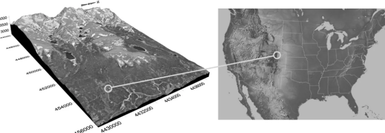
2005). The soils at the forested subalpine zone of the Front Range are typically cryalfs or cryolls depending on slope orientation (Birkeland et al., 2003), developed on glacial till, extremely gravelly (granite debris). During May (spring), when the annual snowmelt occurs, the soils are fairly saturated with melt water. The mountain-valley winds predominate at this site (Fig. 1), upslope flows from the east occur on many summer afternoons bringing high concentrations of anthropogenic pollutants, including ozone, from the Denver/Boulder Metropolitan area and have a profound effect on atmospheric ozone dynamics (Turnipseed et al., 2009). Table 1 contains the descriptive parameters of this site.
Fig. 1. Relief and location of the Niwot Ridge Ameriflux site.
Table 1. Descriptive characteristics of the study site, and site specific model input data used in the calculations
Site characteristics Value Reference
Average annual mean temperature 0.13 °C 1961–1990 mean, CRU CL 2.0 dataset (New et al., 2002) Annual total precipitation 482 mm
Mean (minimum, maximum) temperature (T)
9.41 °C (–14.17 °C, 23.63 °C)
May-October 2003, measured dataset
Total precipitation (P) 232 mm
Mean (minimum, maximum) soil water content (SWC,θ)
0.152 m3 m–3 (0.076 m3m–3, 0.389 m3 m–3) Site specific data used in model
Average height of canopy (h) 11.4 m
(Turnipseed et al., 2009)
Leaf area index (LAI) 4.2 m2 m−2
Displacement height (d) 7.8 m
2.2. Measurements
2.2.1. Data used in the study
Continuous ozone flux and meteorological measurements above a subalpine forest canopy (Pinus contorta, Picea engelmannii, Abies lasiocarpa) were carried out during the growing season (May-October) of 2003 at 21.5 m height.
Effect of short term variations in meteorological parameters has already been discussed in a previous publication (Turnipseed et al., 2009). The ozone flux was measured using the eddy-covariance (EC) technique above the canopy, detailed description of the experiment can be found in Monson et al. (2002) and Turnipseed et al., (2002, 2003, 2009). The meteorological data (air temperature (T), vapor pressure deficit (VPD), soil water content (SWC), photosynthetically active radiation (PAR), and solar radiation (SR) measurements), carbon-dioxide (CO2) flux, and additional information were obtained from the Ameriflux network (cdiac.ornl.gov/ftp/ameriflux/data/). Due to the lack of in-situ measurements of soil water retention, the value of wilting point (0.169 m3 m−3) and field capacity soil moisture (0.396 m3 m−3) were taken from the IGBP-DIS (5×5 arc-minutes) resolution database (Global Gridded Surfaces of Selected Soil Characteristics (International Geosphere-Biosphere Programme – Data and Information System)) (Global Soil Data Task Group).
2.2.2. Data processing and quality assurance
Quality assurance of measured ozone flux data were carried out. Positive fluxes were not taken into account (ozone flux toward the ecosystem is negative by definition). After filtering the ozone flux data, the dataset contains 4013 records of the initially available 5243 half-hourly values (23% of the data were omitted) and 24% of carbon-dioxide fluxes were excluded (initially 7142 data, after filtering 5395). Flux data were omitted during periods of precipitation and very low turbulence intensity, where friction velocity (u*) is less than 0.2 ms–1 after Turnipseed et al. (2009).
In the case where measured data were available for more than 70% of the day (assumed as a representative day), gap filling of measured ozone flux was performed to fill the missing half-hourly values using monthly mean diurnal variations technique (Falge et al., 2001). Using the same technique, daily accumulated ozone fluxes and daily averages of environmental parameters were calculated to eliminate the effect of diurnal variations of wind direction due to the mountain-valley wind system on the days when measured data were available for more than 70% of the day.
2.3. Modeling
The dry deposition models evaluated here are all routinely applied in studies using regional CTMs that are described in the literature and applied over large spatial extents (Stern et al., 2008; Cho et al., 2009), therefore, it is important to examine the accuracy of their estimations. The ZHANG model is the deposition submodel of AURAMS CTM (Smyth et al., 2009), and DEPAC is applied in RCG (Stern, 2009) and in LOTOS-EUROS (Schaap et al., 2008) CTMs. Models were tested in site-specific mode, which employs local vegetation parameters (Table 1) and in situ meteorological observations as input data. Alternatively, the investigated models can be run in regional mode, using the default vegetation parameters, even though these deposition models are not validated for all types of LUCs described by the simulations.
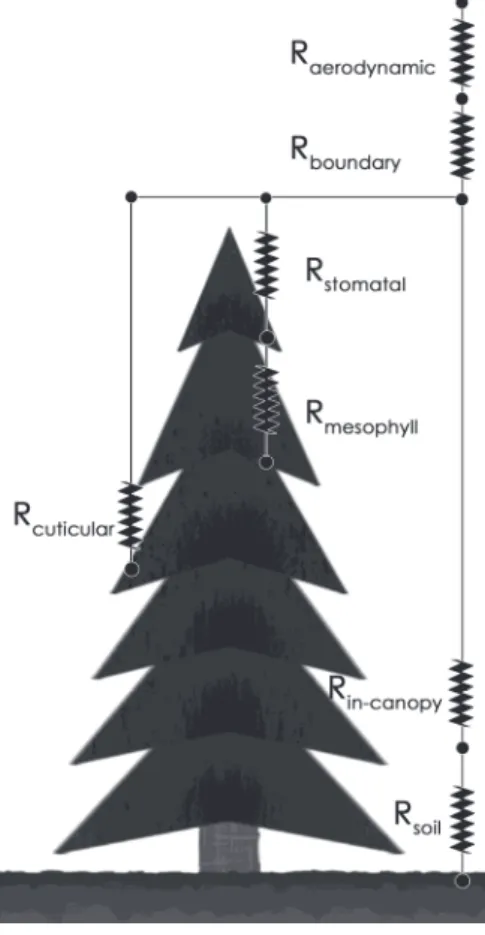
The dry deposition models are vertical (1-dimensional), one-layered models based on the so-called big-leaf concept, as the canopy is treated as one big leaf surface (Fig. 2), and the deposition velocity is calculated using the resistance analogy:
c b
d Ra R R
v = + 1 +
. (2)
Deposition velocity can be calculated as the reciprocal value of the residual of the resistances (analogous to Ohm’s low for electricity) via parameterization of the aerodynamic (Ra) and quasi-laminar boundary layers (Rb) and canopy resistance (Rc), where this latter term includes stomatal (Rst), mesophyll (Rmes), in-canopy (Rinc), cuticular (Rcut), and soil (Rsoil) resistances.
Resistance schemes are described later in Section 2.3. The differences in the schemes occur in parameterization of these resistances (Table 2). Calculation of Ra is very similar in both models, the ZHANG model uses the formula presented in Padro et al. (1991) and the DEPAC model uses the parameterization of Wesely and Hicks (1977). Rb is parameterized using the same formula (Hicks, 1982) in both models. To estimate Rc, the following equations were used in the ZHANG model (Eq.(3), Zhang et al., 2003) and in the DEPAC model (Eq.(4), Erisman et al., 1994):
soil inc
cut mes
st c
1 1 1
1
R R
R R
R W R
st
+ + + +
= − , (3)
soil inc
cut mes
st c
1 1
1 1
R R
R R
R
R + + +
= + , (4)
where Wst is the fraction of stomatal blocking under wet conditions, and is calculated as:
>
≤
− <
≤
=
−
−
−
2 2 2
Wm 600 ,
5 . 0
Wm 600 200
800 , ) 200 (
Wm 200 ,
0
SR SR SR
SR
Wst . (5)
Zhang et al. (2003) stated that in the case of morning dew and sunshine immediately after rain, solar radiation could be strong and Rst is small, however, stomata can be partially blocked by water films and the Wst term will then increase the stomatal resistance.
Fig. 2. Resistance network used in the models.
One of the main differences between the models is the parameterization of stress functions of Rst (Table 2). The ZHANG model calculates Rst as described in Zhang et al. (2002, 2003), meanwhile DEPAC model has two different parameterizations for the stomatal resistance based on Baldocchi et al. (1987) (referred to here as the DEPAC-Baldocchi model) and Wesely (1989) (referred to here as the DEPAC-Wesely model), therefore, three different modules are
used in this study. Both the ZHANG model and the DEPAC-Baldocchi model calculate Rst using functions of air temperature (f(T)) and vapor pressure deficit (f(VPD)), but water stress is described in different ways (for detailed description of model equations see Appendix 1). In the case of optimum environmental conditions, the canopy stress functions are equal to one, representing no stress.
In the ZHANG model, water stress (f(ψ)) is a step function of leaf-water- potential (ψ) depending on SR (Table 2), meanwhile in the DEPAC-Baldocchi model there is no soil water stress, f(θ) equals to 1.
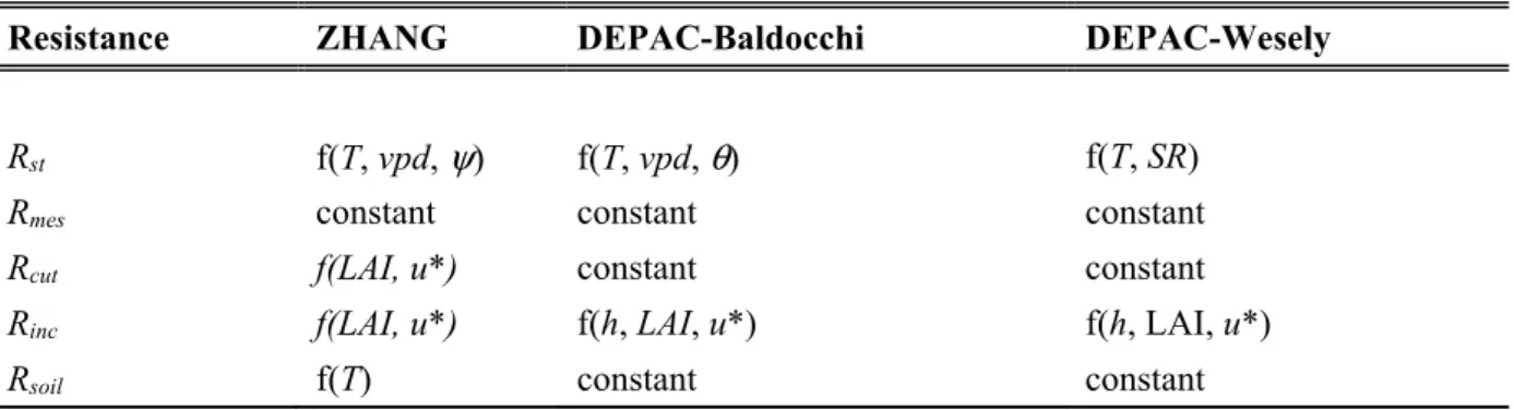
Table 2. Description of main resistances and their parameterization in the model versions used in the study. Independent variables determining their values in the different parameterizations of the models are shown
Resistance ZHANG DEPAC-Baldocchi DEPAC-Wesely
Rst f(T, vpd, ψ) f(T, vpd, θ) f(T, SR)
Rmes constant constant constant
Rcut f(LAI, u*) constant constant
Rinc f(LAI, u*) f(h, LAI, u*) f(h, LAI, u*)
Rsoil f(T) constant constant
Finally, model parameterization improvements were carried out. Many studies have shown that soil moisture is an important factor for controlling stomatal activity (Bates and Hall, 1981; Gollan et al., 1986). It has been shown previously and also acknowledged in the literature that resistance based models are sensitive to moisture stress parameterization (Büker et al., 2012; Van Wijk et al., 2000). Soil moisture content data is easy to obtain compared to the leaf- water-potential used in some modeling approaches. Since none of the investigated models use soil moisture in the parameterization of stomatal resistance, model improvements were carried out (the ZHANG modified model and the DEPAC-Baldocchi modified model later on) with the introduction of a soil moisture (f(θ) in Eq.(6)) stress function based on the work of, e.g., Mészáros et al. (2009) and Grünhage and Haenel (2008). In the case of ZHANG model, the leaf-water-potential function was replaced by a function of soil moisture. In the case of DEPAC-Baldocchi model, instead of constant value (no soil moisture stress), the soil moisture stress function was implemented. The stress function introduced in the models for SWC is as follows:
w f w
f
w f
w
θ θ
θ θ θ
θ θ f
≤
≤
<
>
−
= −
if if
if
05 . 0
05 . 0 , max
1 )
( θ θ
θ
θ θ , (6)
where θw and θf denote soil moisture content corresponding to the wilting point and the field capacity, respectively.
To explore the performance of the different resistance schemes of the investigated models without influence of parameterization of environmental parameters, measured meteorological variables were used when it was possible, and meteorological and astronomical parameterizations (e.g., characteristics of moist air and solar radiation) were synchronized using one common scheme in all other cases. Vapor pressure deficit was calculated using the approach of the World Meteorological Organization (2008), density of moist air, specific heat of moist air was estimated after Grünhage and Haenel (2008). Solar zenith angle was calculated using the parameterization scheme provided by NASA (Landsman, 1993).
2.4. Evaluation methodology 2.4.1. Measurement evaluation
In the first part of this work, analyses of in situ observations were carried out to explore the effect of environmental factors on ozone deposition. Climate impact studies and ecosystem studies are mainly focused on the accumulated pollutant load the ecosystem receives, i.e., the ozone uptake, to be able to qualitatively evaluate/predict its effect on photosynthetic activity (Harmens and Mills, 2012;
Lombardozzi et al., 2012; Tang et al., 2014).
We examined soil moisture, global radiation, photosynthetically active radiation, vapor pressure deficit, and temperature as abiotic controlling factors of ozone flux. Half-hourly measurements were quality checked and analyzed for the whole six-month-long period for changes in relationships between ozone fluxes and ozone deposition drivers throughout the growing season (May- October).
2.4.2. Model evaluation
In the second part of our study, outputs of three deposition models were compared to measured ozone fluxes. Different model quality indicators were calculated to evaluate model performance using half-hourly data on monthly and six-month-long time scales. The statistical metrics used in this study (Pearson linear correlation coefficient (R), mean bias (MB), mean absolute error (MAE),
root mean square error (RMSE), normalized mean square error (NMSE), index of agreement (IA), and modeling efficiency (ME) indicators) were calculated for the whole period both for daytime (when the solar zenith angle is greater than zero) and nighttime (when the solar zenith angle is less than or equal to zero).
The equations of these metrics are given below (Neter et al., 1988; Chang and Hanna, 2004; Pereira, 2004; Falge et al., 2005). R is the linear correlation between the observations and model results, values can vary between −1 and 1 (perfect correlation), 0 means the datasets are independent. MB is a measure of overall bias for variables, in case of perfect estimation it is 0. MAE is overall absolute bias of observed and modeled data. RMSE is the square root of the average squared bias of the modeled data, it is sensitive for extreme errors.
NMSE emphasizes the scatter in the entire data set. Smaller values of NMSE denote better model performance. IA can vary between 0 and 1, and it is a metric of mean square error, in case of perfect agreement it is equal to 1. ME has a range from 1 to −∞, and it is a measure of the accuracy of model estimations to the mean of observations, any positive value means that estimation is better than means of measurements, in case of perfect agreement it is equal to 1.
3. Results and discussion
3.1. Controlling factors of ozone fluxes
In order to explore the effect of environmental factors on ozone deposition, relationships between environmental variables and energy fluxes were examined on a daily basis and on the original half-hourly resolution using eddy covariance (EC) data.
Half-hourly measured meteorological data were compared (T, SWC, VPD, SR, PAR) with half-hourly measured ozone fluxes. Fig. 3 shows time series plots for these variables. The soil at the site was more or less saturated with water during May, therefore, soil moisture is probably not a limiting factor during that period. Turnipseed et al. (2009) found that after photosynthetic photon flux density (PPFD), VPD was the most dominant environmental driver controlling the daytime deposition of O3 at this site through its influence over stomatal conductance.
Fig. 3. Time series of controlling factors and ozone flux (May-October, 2003).
3.2. Results of model evaluations
Model results were investigated on half-hourly and daily time steps, and model performance indicators were calculated based on measured and modelled ozone flux data.
The ZHANG model outperformed the other two model versions on the original half-hourly resolution, but one should be aware of the still poor correlation between measured and modeled ozone flux for the whole period (Table 3). In order to evaluate the average behavior of models and how their performance varies with time of the day, mean diurnal variations of measured and modeled ozone fluxes were calculated. The ZHANG model provided the best results compared to the other two models in capturing the ozone flux magnitude and dynamics as shown by mean diurnal variation (Fig. 4A and C).
The ZHANG modified model in Fig. 4A will be addressed later in the paper.
Table 3: Model quality indicators based on half-hourly measured ozone fluxes (May-October, 2003)
Model
name Period R2
(p<0.001) N MB
[nmol m–2 s–1]
MAE
[nmol m–2 s–1]
RMSE
[nmol m–2 s–1]
NMSE
[nmol m–2 s–1]
IA ME
ZHANG model
All data 0.26 3877 1.39 3.21 4.45 0.52 0.68 0.08
Daytime 0.17 2796 1.83 3.77 4.91 0.44 0.59 –0.03
Nighttime 0.07 1081 0.25 1.76 2.91 0.93 0.47 –0.15
DEPAC- Baldocchi model
All data 0.15 3877 7.30 8.09 10.07 1.44 0.46 –3.71
Daytime 0.05 2796 9.84 10.47 11.72 1.29 0.37 –4.88
Nighttime 0.02 1081 0.74 1.93 2.90 0.80 0.31 –0.15
DEPAC- Wesely model
All data 0.07 3877 –0.50 3.03 4.55 0.75 0.42 0.04
Daytime 0.01 2796 –0.98 3.46 5.04 0.70 0.34 –0.09
Nighttime 0.02 1081 0.74 1.93 2.90 0.80 0.31 –0.15
Mean measured ozone flux [nmol m–2 s–1] for all data: –5.50, daytime: –6.51, nighttime: –2.90
Fig. 4. Performance of the ZHANG model and the ZHANG modified model (May- October, 2003): (A) mean diurnal variation of half-hourly measured and modeled ozone flux, (B) daily accumulated measured and modeled ozone flux. Performance of the DEPAC-Baldocchi model, the DEPAC-Wesely model, and the DEPAC-Baldocchi modified model (May-October, 2003): (C) mean diurnal variation of half-hourly measured and modeled ozone flux, (D) daily accumulated measured and modeled ozone flux.
The performances of the two versions of the DEPAC model stay below that of the ZHANG model as it is reflected by most model quality indicators listed in Table 3. Correlation is lower, the DEPAC-Baldocchi and the DEPAC-Wesely parameterization can only explain 15% and 7% of the observed variance. Model errors are significantly higher in the case of the DEPAC-Baldocchi parameterization. It should be noted that although DEPAC-Wesely can explain even less of the observed variance of half-hourly ozone deposition, its performance is comparable to that of the ZHANG model based on some other statistical measures (IA, ME, NMSE, RMSE).
Mean diurnal variation of ozone deposition modeled by different parameterizations of the DEPAC model are shown in Fig. 4C together with measured ozone deposition. The DEPAC-Baldocchi model overestimates the measured fluxes (as it is also indicated by statistics based on the full half-hourly dataset, shown in Table 3). The most important difference between the ZHANG and DEPAC models lies in the parameterization of Rst. It has been reported by Mészáros et al. (2009) that deposition models are sensitive to soil moisture content input. The soil moisture stress is not parameterized in the DEPAC- Baldocchi model, f(θ) has a fixed value of one, which assumes that there is no water stress for the canopy. So, these results show that it is essential to include the soil moisture in the dry deposition models, consequently, the ZHANG model is to be preferred above the DEPAC models.
As it is presented in Fig. 4C, the DEPAC-Wesely model underestimates the measured fluxes, although model error is lower than in the case of the DEPAC- Baldocchi parameterization (Table 3). The DEPAC-Baldocchi modified model in Fig. 4C will be discussed later in the paper.
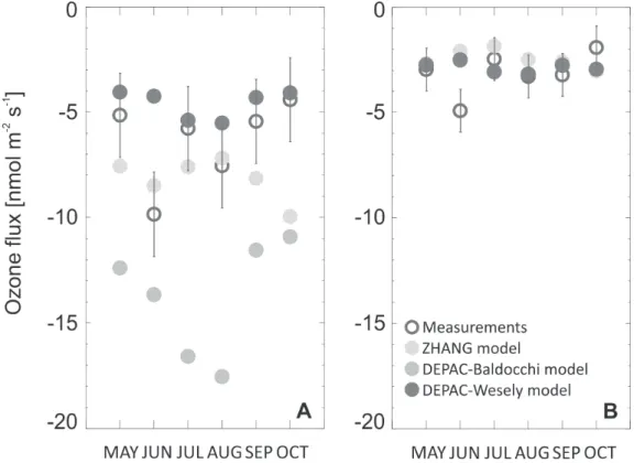
To explore if models capture long-term variabilities, monthly means of ozone fluxes were calculated (Fig. 5). We separated data to daytime (when solar elevation angle is greater than 0, Fig. 5A) and nighttime (when solar elevation angle is less than 0, Fig. 5B) parts, since the modeling approach is different for nighttime conditions (see Appendix 1). The calculated nighttime ozone deposition data reveal a very good agreement with measured flux (Fig. 5B). Considering that nighttime ozone fluxes are dominated by cuticular or soil pathways, this good performance compared to the daytime performance of the models suggests that mostly the description of stomatal uptake is responsible for model errors. For observed ozone flux during nighttime, the DEPAC-Baldocchi and the DEPAC-Wesely models result in the same values, since the parameterizations are the same for nighttime conditions. For daytime data where stomatal resistance is calculated using the more sophisticated approach described in Appendix 1, model performances diverge more.
The relatively simple parameterization of the DEPAC-Wesely model simulated monthly average ozone deposition with the smallest bias in each month except June. It should be kept in mind, however, that only measured ozone flux data is considered here, i.e., this is not real average ozone deposition but the monthly average of available measured data.
When models are applied in climate change impact studies over large spatial and temporal extents, data are often not used in their original temporal resolution (see, e.g., Sitch et al., 2007). Model results were examined on a daily time step using accumulated ozone fluxes to simulate ozone load (Fig. 4B, Fig. 4D). This approach is used in most large scale climate impact studies.
Results of the ZHANG model have the best correlation with the measured accumulated ozone fluxes (R2 = 0.23, p < 0.05, Table 4), but in case of DEPAC- Baldocchi, the model correlation cannot be detected (R2 = 0.05, p = 0.144, Table 4).
Fig. 5. Monthly means of half-hourly modeled and measured ozone fluxes (May-October, 2003): (A) daytime, when solar elevation greater than 0, (B) nighttime, when solar elevation is less than zero. Standard deviation of measured data is also shown as error bars.
Table 4. Model quality indicators based on daily measured accumulated ozone fluxes (May-October, 2003)
Model
name R2 p N MB [μmol m–2 day–1]
MAE [μmol m–2 day–1]
RMSE [μmol m–2 day–1]
NMSE [nmol m–2 day–1]
IA ME ZHANG
model 0.22 0.002 39 148.92 171.07 218.66 0.28 0.99 0.96 DEPAC-
Baldocchi model
0.06 0.144 39 548.17 552.93 585.12 1.13 0.98 0.51 DEPAC-
Wesely model
0.02 0.358 39 61.14 119.43 151.74 0.17 1.00 0.99
Mean measured ozone flux [μmol m–2 day–1]: –340.94
This contradicting behavior of the three structurally identical models demonstrates the need for a careful interpretation of resistance based model results for sites where no previous results are reported in the literature regarding correlation and systematic model errors. Results of the ZHANG modified model (Fig. 4A) has a lower correlation (R2 = 0.09, p < 0.001 instead of 0.25 in Table 3) with measurements using the full half-hourly dataset, and RMSE value did not change (4.69 nmol m−2 s−1). In case of the DEPAC-Baldocchi modified model (Fig. 4C), R2 decreased (0.05, p < 0.001 instead of 0.15 in Table 3), parallel RMSE decreased almost by half compared to the original parameterization (4.66 nmol m−2 s−1 versus 10.07 nmol m−2 s−1). On a daily time step, the DEPAC-Baldocchi modified model results showed better correlation with measured accumulated ozone fluxes than the original model (R2 = 0.06, p = 0.140; Fig. 4D). Comparing Fig. 4B and Fig. 4D we can conclude that the modified models resulted in similar values, at least compared to the differences observed when comparing the original model versions. This can be explained by non-stomatal resistance (Rcut, Rinc, and Rsoil), since with implementation of f(θ), Rst has the same value in both modified models.
Mészáros et al. (2009) carried out a sensitivity analysis of a multiplicative dry deposition model and found that soil moisture content is one of the most influential parameters in the model. This explains why the introduction of soil moisture stress parameterization in the DEPAC-Baldocchi model had such a dramatic effect on model results. However, as indicated by measurements, soil moisture was not a driving factor for ozone deposition at this site in the measurement period. This suggests that model constraints do not reflect real environmental circumstances, i.e., model results agree with measured ozone fluxes, but the model fails to explain short-term variability of ozone deposition, which led to a decrease in correlation between half-hourly measured and modeled ozone fluxes. The use of soil moisture content data representative for the whole root zone when available should improve model results.
4. Conclusion
In this study, ecosystem-atmosphere ozone fluxes are simulated using three widely used deposition models. Our model validation results showed worse model performance during daytime when stomatal activity is higher, which suggests that modeling problems are especially related to the stomatal pathway ozone deposition. It was also shown that the ZHANG model is to be preferred under most circumstances, as it provided the best model-measurement agreement among the used models in hourly and daily time steps. Nevertheless, the most accurate long-term (monthly average) results were provided by the DEPAC-Wesely model. The inclusion of soil moisture stress in two models improved model accuracy, but the correlation remained low, suggesting that
there are other errors in the description of factors and their interactions regulating ozone deposition in the models.
In spite of their wide acceptance (Brook et al., 1999; Flemming and Stern, 2007), the multiplicative models used in this study have not been calibrated for some important land cover types, e.g., none of the above models have been calibrated for evergreen forests. In studies where these models are applied on large spatial scales, continents, and countries (Manders et al., 2012; van Loon et al., 2007; Smyth et al., 2009), this can bias the results over these land uses, leading to spatially varying uncertainty in the estimations, which should be considered when interpreting results from chemical transport models. According to our results, even if we minimize input data errors using measured driving data when available, model results diverge when validated for a randomly selected geographical location and land use type. This suggests, that the lack of calibration inhibits the reliable use of these models in case of ecosystem types other than they have been calibrated for, and hence, their practicality in large scale studies, where models are used over several ecosystems, might be questionable and their results should be interpreted carefully.
Acknowledgement: The authors would like to thank Prof. Russell Monson and the Niwot Ridge AmeriFlux site for access to their data. Present article was published in the frame of the project TÁMOP-4.2.2.A- 11/1/KONV-2012-0064. The project is realized with the support of the European Union, with the co- funding of the European Social Fund. This research was funded by the TÁMOP/SROP-4.2.2.C- 11/1/KONV-2012-0005 Scholarship (Well-being in the Information Society) Grant.
The authors declare that there is no conflict of interests regarding the publication of this paper.
Appendix
Appendix 1: Formulas used in the model to describe the resistance network.
Zhang model DEPAC model
−
⋅
= ⋅ r h
a z
z
R u ψ
κ1 * 0.74 ln 0
−
= ⋅ r h
a z
z
R u ψ
κ * ln 0 1
*
31 5 .
1 u
Rb = ⋅
637 . 0 ) ( ) ( )
(
1
⋅
⋅
⋅
= ⋅
ψ f vpd f f(T) PAR R G
st st
Baldocchi
637 . 0 ) ( ) ( )
(
1
⋅
⋅
⋅
= ⋅
θ f vpd f f(T) PAR R G
st st Wesely
+ +
− ⋅
⋅ ⋅
⋅
=
2
1 . 0 1 200
) 40 ( 571 400
,
1 R T T SR
Rst i
if solar elevation < 0: Rst = 12500
[ ]
sm–1[ ]
sm–1=0 Rmes
cut RH
e LAI
R u
03 . 0 25 . 0
*
4000
⋅
= ⋅
if T < −1˚C: Rcut =Rcut⋅e0.2(−1−T) Rcut =1000
[ ]
sm–12
* 25 . 0
) ( 100
u
Rinc = ⋅LAI 8 *
u h LAI Rinc = ⋅ ⋅
[ ]
sm–1=200 Rsoil
if T< −1˚C:
) 1 ( 2 .
0 T
soil
soil R e
R = ⋅ − −
[ ]
sm–1=100 Rsoil
if T< 0˚C: Rsoil = 2000
[ ]
sm–1( ) ( ) st( sh)
sh s
st st s
PAR r
LAI PAR
r PAR LAI
G = + Gst
(
PAR)
= 250⋅(
1+25LAI/PARmeasured)
(
x) (
x)
st PAR PAR
r =250⋅ 1+25/
[ ] [ ] [ ] [ ]
=
spring sm
250
winter sm
400
autumn sm
250
summer sm
130
1 –
1 –
1 –
1 –
Ri
) ( 1
)
(VPD b e e
f = − VPD⋅ s −
bT
opt
opt T T
T T
T T
T T T
f
−
⋅ −
−
= −
max max min
) min
(
, Baldocchi et al., 1987
min max
max
T T
T bT T opt
−
= −
, Baldocchi et al., 1987
2 1 2
1
2 1
2
if if
if
05 . 0
05 . 0 , max
1 )
(
c c c
c
c c
f c
ψ ψ
ψ ψ ψ
ψ ψ ψ
ψ ψ ψ ψ
≤
≤
<
>
−
= −
SR 0013 . 0 72 .
0 −
− ψ =
1 ) (θ = f
unstable
⋅
− +
⋅
= 2
9 1 1 ln 74 . 0
25 . 0
L z Φ
r h
unstable
−
⋅
−
−
⋅ +
=
2
ln 09 . 0 ln
39 . 0 598 . 0
exp L
z L
Φh zr r
stable L Φh =−4.7zr
stable L Φh=−5zr
neutral
=0 Φh
Appendix 2: Nomenclature for Appendix 1.
ψc1, ψc2 specify leaf-water-potential dependency parameters [MPa]
Φh dimensionless stability function bVPD vpd constant [kPa−1],
e, es ambient and saturation water vapor pressure [kPa], respectively Gst unstressed stomatal conductance [m s–1]
κ Karman constant (0.41)
L Monin-Obukhov length (calculation method is not detailed here) [m]
PARs/PARsh PAR received by sunlit and shaded leaves, respectively [W m–2] Ri minimum bulk canopy stomatal resistances for water vapor [s m–1] rst unstressed leaf stomatal resistance [s m–1]
Tmin, Tmax, Topt minimum, maximum and optimum T for stomatal opening, respectively(–5 °C, 40 °C and 15 °C)
zr reference height [m]
References
Anav, A., Menut, L., Khvorostyanov, D., and Viovy, N., 2011: Impact of tropospheric ozone on the Euro-Mediterranean vegetation. Glob. Change Biol. 17, 2342–2359.
https://doi.org/10.1111/j.1365-2486.2010.02387.x
Ashmore, M.R., 2005: Assessing the future global impacts of ozone on vegetation. Plant Cell Environ.
28, 949–964. https://doi.org/10.1111/j.1365-3040.2005.01341.x
Baldocchi, D.D., Hicks, B.B., and Camara, P., 1987: A canopy stomatal resistance model for gaseous deposition to vegetated surfaces. Atmos. Environ. 21, 91–101.
https://doi.org/10.1016/0004-6981(87)90274-5
Ball, J.T., Woodrow, I.E., and Berry, J.A., 1987: A model predicting stomatal conductance and its contribution to the control of photosynthesis under different environmental conditions, In (ed.:
J. Biggens) Progress in Photosynthesis Research, IV. Martinus Nijhoff, Dordrecht, 221–224.
https://doi.org/10.1007/978-94-017-0519-6_48
Bates, L.M. and Hall, A.E., 1981: Stomatal Closure with Soil-Water Depletion No Associated with Changes in Bulk Leaf Water Status. Oecologia 50, 62–65. https://doi.org/10.1007/BF00378794 Bey, I., Jacob, D.J., Yantosca, R.M., Logan, J.A., Field, B., Fiore, A.M., Li, Q., Liu, H., Mickley, L.J.,
and Schultz, M., 2001: Global modeling of tropospheric chemistry with assimilated meteorology: Model description and evaluation. J. Geophys. Res, 106, 23073–23095.
https://doi.org/10.1029/2001JD000807
Birkeland, P.W., Shroba, R.R., Burns, S.F., Price, A.B., and Tonkin, P.J., 2003: Integrating soils and geomorphology in mountains–an example from Front Range Colorado. Geomorphology 55, 329–344 https://doi.org/10.1016/S0169-555X(03)00148-X
Brook, J.R., Zhang, L., Li, Y., and Johnson, D., 1999: Description and evaluation of a model of deposition velocities for routine estimates of dry deposition over North America. Part II: review of past measurements and model results. Atmos. Environ. 33, 5053–5070.
Büker, P., Emberson, L.D., Ashmore, M.R., Cambridge, H.M., Jacobs, C.M.J., Massman, W.J., Müller, J., Nikolov, N., Novak, K., Oksanen, E., Schaub, M., and de la Torre, D., 2007: Comparison of different stomatal conductance algorithms for ozone flux modelling. Environ. Pollut. 146, 726–735.
https://doi.org/10.1016/j.envpol.2006.04.007
Büker, P., Morrissey, T., Briolat, A., Falk, R., Simpson, D., Tuovinen, J.-P., Alonso, R., Barth, S., Baumgarten, M., Grulke, N., Karlsson, P. E., King, J., Lagergren, F., Matyssek, R., Nunn, A., Ogaya, R., Peñuelas, J., Rhea, L., Schaub, and M., Uddling, 2012: DO3SE modelling of soil moisture to determine ozone flux to forest trees. Atmos. Chem. Phys. 12, 5537–5562.
https://doi.org/10.5194/acp-12-5537-2012
Chamberlain, A.C., 1967: Transport of Lycopodium Spores and Other Small Particles to Rough Surfaces. Proceedings of the Royal Society of London, Series A, Mathematical and Physical Sciences 296, 45–70. https://doi.org/10.1098/rspa.1967.0005
Chang J.C. and Hanna, S.R., 2004: Air quality model performance evaluation. Meteorol. Atmos. Phys.
87, 167–196. https://doi.org/10.1007/s00703-003-0070-7
Cho, S., Makar, P. A., Lee, W. S., Herage, T., Liggio, J., Li, S. M., Wiens, B., and Graham, L., 2009:
Evaluation of a unified regional air-quality modeling system (AURAMS) using PrAIRie2005 field study data: The effects of emissions data accuracy on particle sulphate predictions. Atmos.
Environ. 43, 1864–1877. https://doi.org/10.1016/j.atmosenv.2008.12.048
Emery, C., Jung, J., Downey, N., Johnson, J., Jimenez, M., Yarwood, G., and Morris, R., 2012:
Regional and global modeling estimates of policy relevant background ozone over the United States. Atmos. Environ. 47, 206-217. https://doi.org/10.1016/j.atmosenv.2011.11.012
Erisman, J., Van Pul, A., and Wyers, P., 1994: Parameterization of surface resistance for the quantification of atmospheric deposition of acidifying pollutants and ozone. Atmos. Environ. 28, 2595–2607. https://doi.org/10.1016/1352-2310(94)90433-2
Falge, E., Baldocchi, D., Olson, R., Anthoni, P., Aubinet, Marc, Bernhofer, C., Burba, G., Ceulemans, R., Clement, R., Dolman, H., Granier, A., Gross, P., Grunwald, T., Hollinger, D., Jensen, No., Katul, G., Keronen, P., Kowalski, A., Lai, Ct., Law, Be., Meyers, T., Moncrieff, H., Moors, E., Munger, Jw., Pilegaard, K., Rannik, U., Rebmann, C., Suyker, A., Tenhunen, J., Tu, K., Verma, S., Vesala, T., Wilson, K., and Wofsy, S., 2001: Gap filling strategies for defensible annual sums of net ecosystem exchange. Agr. Forest Meteorol. 107, 43–69.
https://doi.org/10.1016/S0168-1923(00)00225-2
Falge, E., Reth, S., Brüggemann, N., Butterbach-Bahl, K., Goldberg, V., Oltchev, A., Schaaf, S., Spindler, G., Stiller, B., Queck, R., Köstner, B., and Bernhofer, C., 2005: Comparison of surface energy exchange models with eddy flux data in forest and grassland ecosystems of Germany.
Ecol. Model. 188, 174–216. https://doi.org/10.1016/j.ecolmodel.2005.01.057
Fares, S., Vargas, R., Detto, M., Goldstein, A., Karlik, J., Paoletti, E., and Vitale, M., 2013:
Tropospheric ozone reduces carbon assimilation in trees: estimates from analysis of continuous flux measurements. Glob. Change Biol. 19, 2427–2443. https://doi.org/10.1111/gcb.12222 Flemming, J. and Stern, R., 2007: Testing model accuracy measures according to the EU
directives – examples using the chemical transport model REM-CALGRID. Atmos.
Environ. 41, 9206–9216. https://doi.org/10.1016/j.atmosenv.2007.07.050
Fowler, D., Amann, M., Anderson, R., Ashmore, M., Cox, P., Depledge, M., Derwent, D., Grennfelt, P., Hewitt, N., Hov, O., Jenkin, M., Kelly, F., Liss, P., Pilling, M., Pyle, J., Slingo, J., and Stevenson, D., 2008: Ground-level ozone in the 21st century: future trends, impacts and policy implications. Royal Society Policy Document 15/08, London: The Royal Society.
Global Soil Data Task Group. Global Gridded Surfaces of Selected Soil Characteristics (IGBP-DIS).
Data set. Available on-line [http://www.daac.ornl.gov] from Oak Ridge National Laboratory Distributed Active Archive Center, Oak Ridge, Tennessee, U.S.A.
https://doi.org/10.3334/ORNLDAAC/569
Gollan, T., Passioura, J.B., and Munns, R., 1986: Soil-Water Status Affects the Stomatal Conductance of Fully Turgid Wheat and Sunflower Leaves. Aust. J. Plant Physiol. 13, 459–464.
https://doi.org/10.1071/PP9860459
Grell, G.A., Peckham, S.E., Schmitz R., S.A., McKeen, Frost, G., Skamarock, W.C., and Eder, B., 2005: Fully coupled 'online' chemistry in the WRF model. Atmos. Environ.t 39, 6957–6976.

![Table 3: Model quality indicators based on half-hourly measured ozone fluxes (May-October, 2003) Model name Period R 2 (p<0.001) N MB [nmol m –2 s –1 ] MAE [nmol m–2 s–1] RMSE [nmol m–2 s–1] NMSE [nmol m–2 s–1] IA ME ZHANG model All d](https://thumb-eu.123doks.com/thumbv2/9dokorg/1426355.121060/13.892.92.772.587.856/table-model-quality-indicators-hourly-measured-october-period.webp)