DOI:10.28974/idojaras.2018.3.5
IDŐJÁRÁS
Quarterly Journal of the Hungarian Meteorological Service Vol. 122, No. 3, July – September, 2018, pp. 305–320
Application of the crop model WOFOST in grid using meteorological input data from reanalysis and
objective analysis
Hristo Chervenkov*, Valentin Kazandjiev, and Veska Gorgieva
National Institute of Meteorology and Hydrology, Bulgarian Academy of Sciences
66, Tsarigradsko Shose blvd Sofia 1784, Bulgaria
* Corresponding author Email: Hristo.Tchervenkov@meteo.bg
(Manuscript received in final form June16, 2017)
Abstract⎯Meteorological gridded datasets from the reanalysis ERA-Interim of the ECMWF and the objective analysis E-OBSv14.0 of the ECA&D are used to initialize the crop model WOFOST. The data is on daily basis with 0.25° horizontal resolution and the model domain entirely covers southeastern part of Europe. Hence, the general of the authors goal is to investigate the response of the crops system to the averaged weather conditions, rather than of a particular year. For this purpose, multi-year daily averages from the 30-year period of 1981–2010 are considered. This time-span is often treated as
“modern climate”, and it is frequently used in many evaluation studies. A special, purpose-build software system is designed to perform the simulation, which steers the data flow and the exchange between the different modules. The produced outcome, in form of three-dimensional digital map of the crop production specific variables, shows high spatial and temporal consistency, revealing the relevant features of the geographical and chronological variation of the output parametersat the same time.
Key–words: ERA-Interim, E-OBS, WOFOST, crop simulation in grid
1.Introduction
Continued pressure on agricultural land, food insecurity, and required adaptation to climate change has made integrated assessment and modelling of future agro- ecosystems development increasingly important. Various modelling tools are
used to support the decision making and planning in agriculture, and consequently, many common efforts are dedicated to the problem. Thus, for example, the ACCELERATES project (Rounsevell et al., 2006) aimed to assess the vulnerability of European agro-ecosystems to environmental change in support of the conventions of climate change and biological diversity. This was based on a study of the impact of environmental change on land use and biodiversity (for selected species and habitats) in agro-ecosystems. The approach integrated existing models of agricultural land use, species distribution, and habitat fragmentation within a common scenario framework, so that impacts could be synthesized for different global change problems. The results suggest that policy and conservation strategies should not tackle the vulnerability of agriculture and biodiversity independently.
An important component in this is crop modelling. The crop model (CM) simulates or imitates the behavior of a real crop by predicting the growth of its components, such as leaves, roots, stems, and storage organs as a function of the soil and weather conditions and crop-specific parameters. Thus, a CM does not only predict the final state of crop production or harvestable yield, but also contains quantitative information about major processes involved in the growth and development of the crop. Reactions and interactions at the level of tissues and organs are combined to form a picture of the crop’s growth processes. In crop growth modelling, current knowledge of plant growth and development from various disciplines, such as crop physiology, agrometeorology, soil science and agronomy, are integrated in a consistent, quantitative, and process-oriented manner (Oteng-Darko et al., 2013).
Meteorological conditions are the main abiotic factors for the development of the cultivars, and correspondingly, agriculture is influenced by the prevailing weather and climate. Thus, for example, elevated temperature and humidity affect the biological processes like respiration, photosynthesis, plant growth, reproduction, water use, and other processes. Consequently, the quality and reliability of the meteorological input data for the CMs are of primary importance. The most modern CMs are one dimensional, namely they use the meteorological and soil data measured in certain point of interest. According to the meteorological input, the typical and most widely used source of such information, the time series are collected in the network of the standard measurement stations. Obviously, the resulted CM output is spatially limited also to the vicinity of the location of the point of the information source. An alternative approach is to use meteorological data from reanalysis (RA) and objective analysis (OA) and to run the CM gridcell-by-gridcell independently.
The main advantage of the RA and OA is obvious: they provide spatially and temporally the best estimated picture of the state of the atmosphere in form of continuous gridded digital maps. The methods incorporated in every RA model maintain also the dynamical consistency between the variables. The OA, which is, generally speaking, a multistage procedure of error-detecting and removing,
as well as, homogenization and interpolation of the measurements, produces output, which is much more reliable in comparison with the row data.
Consequently, such gridded datasets are widely used and will continue to be important for many reasons (see Haylock et al., 2008 for details). The main aim of the presented work is to investigate the principal applicability of RA and OA datasets for initialization of 'state-of-the-art' CM and to analyze the resulted crop model output. For this purpose, a software system is build, which uses data from the current reanalysis of the European Centre for Medium-Range Weather Forecasts (ECMWF) ERA-Interim and from the version 14.0 of the OA data-set E-OBS of the European Climate Assessment&Dataset (ECA&D) for initialization of the version 7.1.7 of the CM WOFOST. Multi-annual daily averages of the input parameters for the time span 1981–2010 are used, and the model domain covers Southeast (SE) Europe entirely.
The aim of the study is to investigate the crop response to the atmospheric conditions, and more specifically, to the climate means, thus, only the meteorological input is altered. All other input settings and parameters of the CM WOFOST are left on their default values. Thus, generally speaking, the work is a preliminary but necessary prerequisite for more realistic simulations.
The article is structured as follows. Section 2. is dedicated to the concise description of the CM WOFOST, the input datasets and the accepted methodology. Section 3. presents the performed calculations and the obtained results. The conclusion and outlook for the further plans are given in the last section.
2.CM WOFOST, input data and methodology 2.1. CM WOFOST
The CM WOFOST (acronym of WOrld FOod STudies) is created by the school of C.T. De Wit at the Wageningen University in the Netherlands as a successor of earlier simulators. It is a mechanistic model that explains the growth of annual crops on the basis of the underlying processes, such as photosynthesis, respiration, and how these processes are influenced by environmental conditions. The model is intended to facilitate the computation of the annual crop production, biomass, water use, etc. for a given location and knowledge about soil type, crop type, weather data, and crop management factors, e.g., sowing date, cultivation, and fertilization (Eitzinger et al., 2009).
The major processes are phenological development, CO2-assimilation, transpiration, respiration, partitioning of assimilates to the various organs, and dry matter formation. Potential production and two levels of limited production (water-limited and nutrient-limited) can be calculated. Potential production represents the absolute production ceiling for a given crop grown in a given area
current study. Production-reducing factors (like weed and pests) have not been taken into account.
Like all mathematical models of agricultural production, WOFOST is a simplification of the reality. Basically, crop yield is a result of the interaction of ecological, technological, and socio-economical factors. In WOFOST, only ecological factors are considered under the assumption that optimum management practices are applied. Crop rotation and soil cultivation effects are not considered.
The key point is, as stated above, that WOFOST is a one-dimensional simulation model, i.e., without reference to any geographic scale. Its application to regions relies on the selection of representative points. Nevertheless, the WOFOST model was calibrated in Bulgaria and used for prediction of crop growing, development, and yields in operational agrometeorological practice in NIMH-BAS (Kazandjiev and Georgieva, 2006). We are also familiar with other CMs, such as the freely distributed AquaCrop and DSSAT, which is not distributed free of charge. We have adapted one and the other, but we have stopped on WOFOST, because it is the basis of the EC-Crop Growth Monitoring System (CGMS).
In the last two decades, the successive WOFOST versions and their derivatives have been used in many studies around the world including Bulgaria (Kazandjiev and Georgieva, 2006). WOFOST is a significant component of the BioMA (Biophysical Models Applications) software framework of the MARS (Monitoring Agricultural ResourceS, see https://ec.europa.eu/jrc/en/mars for details) initiative of the EU Joint Research Centre (JRC). Main aim of the initiative is to perform regular crop yield forecasting in order to provide monthly bulletins forecasting crop yields to support the EU's Common Agriculture Policy (CAP). Crop yield forecasts and crop production estimates are necessary at EU and Member State level to provide the EU’s CAP decision makers with timely information for rapid decision-making during the growing season. Estimates of crop production are also useful in relation to trade, development policies, and humanitarian assistance linked to food security (Leo and Baruth, 2013).
Variation in timing of crop production can be taken into account by varying the starting date of the growing season and/or by selecting crop cultivars with different growth durations. WOFOST offers several options for positioning the crop calendar in the year. The start of the simulation can be at a fixed date of crop emergence, at a fixed date of sowing, or at a variable date of sowing. The end of the simulated season is determined by crop maturity or crop death, or set at a fixed end date, e.g., for crops harvested immature.
More in-depth information for the model can be found in the user's guide (Boogaard et al., 1998), which ships together with the free-available distributive.
Crop growth is simulated using daily weather data of many years and different parameters for each relevant soil type within a region. If required for a
particular study, calculated values, e.g., yields, biomasses produced, or water use can be averaged over the simulated years or aggregated over soil types.
However, the data needed in this procedure are not always available. The scarcity of the daily weather data is emphasized in the user's guide (Boogaard et al., 1998). It is also stated, that the option included in the model, which uses average (monthly) weather data has to be treated carefully: the use of long-term mean monthly weather data, mean sowing dates, and averaged soil data as model input may lead to a false impression of the agro-ecological potential of a region. This implies that original rather than averaged data must be used as model input, and that if needed, averaging can be done only after the simulation.
The temporal and spatial discontinuity of the point measurements is inherent weakness of each dataset, containing such data. Further and very relevant problem is the absence of such a key agrometeorological parameter from the standard (i.e., synoptic) measurements. Usually, to overcome this, empirical and semi-empirical relations between various parameters, for example, sunshine duration, latitude, longitude from one side, and insolation from the other are implemented. Such relations, as a whole, are very schematic, and their suitability in the crop modelling is disputable. This fact was an additional motivator for the authors to implement OA and RA data for the initialization of the CM WOFOST.
2.2. RA ERA-Interim, OA E-OBS, and used methodology
The latest operational RA of the ECMWF ERA-Interim (Dee et al., 2011) is the global atmospheric reanalysis from 1979, continuously updated in real time. The data assimilation system used to produce ERA-Interim is based on a 2006 release of the Integrated Forecasting System (IFS) (Cy31r2). The system includes a 4-dimensional variational analysis (4D-Var) with a 12-hour analysis window. The spatial resolution of the dataset is approximately 80 km (T255 spectral) on 60 vertical levels from the surface up to 0.1 hPa. ERA-Interim products are updated once per month with a delay of two months, and are freely available via the ECMWF Public Datasets web interface or from the archiving system.
ERA-Interim-driven crop simulations with WOFOST were performed in the in-depth pan-European study of de Wit et al. (2010). In this study, two model setups are considered using two identical model implementations: one uses interpolated observed weather, the other is built from ERA-Interim. Output for both sources was generated for the EU27 and neighboring countries and 14 crops, aggregated to national level and validated using reported crop yields from the European Statistical Office (EUROSTAT). The results indicate that the system performs very similar in terms of crop yield forecasting skill. The other main conclusion of the work is that the ERA-Interim dataset is highly suitable
for regional crop yield forecasting over Europe, and may be used for implementing regional crop forecasting over data-sparse regions.
E-OBS is a land-only daily gridded observational dataset for precipitation amount, minimum, mean, and maximum temperature, and sea level pressure in Europe based on the collected information at ECA&D stations (Haylock et al., 2008). The current version 14.0 covers the period from January 1, 1950 until August 31, 2016. Data is made available on a 0.25 and 0.5° regular latitude- longitude grid, as well as on a 0.22 and 0.44° rotated pole grid, with the North Pole at 39.25N, 162W. In the current implementation, data on the regular 0.25°
regular latitude-longitude grid are used. Besides the 'best estimate' values, separate files are provided containing daily standard errors and elevation.
The weather dataset, necessary for the initialization of the CM WOFOST, must contain the time series of the following six variables: irradiation, minimum temperature, maximum temperature, early morning (EM) vapor pressure, mean wind speed at 2 m above ground, and precipitation. The time steps of all variables, except the vapor pressure, have to be one day, and the latter obviously requires sub-daily time resolution. Practically, the only reliable source of such information is the state-of-the-art RA, and this fact, in conjunction with the need for radiation data, was the main reason to use ERA-Interim. Thus, the data for the EM vapor pressure and mean wind speed are taken from ERA-Interim, while the minimum and maximum temperature, as well as the precipitation amount are from E-OBS.
Although WOFOST is supplied with additional MICROSOFT WINDOWS® graphical user interface, it can be executed as stand-alone console application. In the latter case, all initial data have to be in the required format of the crop, soil, and weather files. The fact, that the FORTRAN-77 source code is freely available is of key importance. Alongside other benefits, this allows the model to be recompiled and linked again and integrated in other, purpose-built software projects, as described in detail in the next section.
3.Performed calculations and obtained results
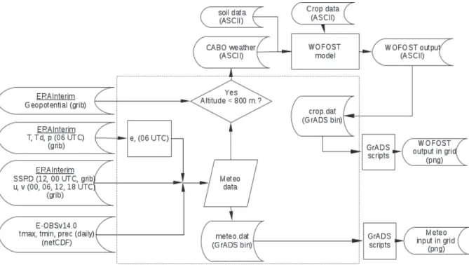
The main aim of the authors was to exploit WOFOST in Unix-like environment, which offers superior opportunities for geophysical modelling. Thus, the model is recompiled and linked under Linux Slackware, using the bash shell script available in the WOFOST distributive. The WOFOST execution, data flow and the linkage between the separate modules are governed from the main, purpose- build program. It is written by the authors in FORTRAN 90/95, and its skeleton is shown as a flow-chart in Fig. 1.
Fig. 1. Building blocks, file formats, and data flow in the simulation system.
The main goal of the authors was to investigate the response of the agricultural system of averaged meteorological conditions rather than of a particular year. Thus, the multi-annual daily averages from the 30-year period 1981–2010 have been considered. All parameters, which are needed for the WOFOST initialization, have been calculated first for every day in the considered period, and the climate averages have been obtained afterward.
The model domain comprises Southeast (SE) Europe and is centered over Bulgaria. It is situated between the 15°and 35° eastern longitudes and the 35°
and 50° northern latitudes and consists of 81×61 0.25×0.25° gridcells.
To ensure the spatial conformability between the ERA-Interim and E-OBS, the ERA-Interim datasets are downloaded with 0.25° resolution.
The variables, needed for the calculation of the water vapor pressure, noted in Fig. 1 with e, namely the temperature T, dew point Td, and surface pressure p, are available in ERA-Interim at 00, 06, 12, and 18 UTC, and thus 06 UTC data are selected as closest to “early morning”. The vapor pressure is obtained with well-known relations, and the results are validated with independent humidity calculators.
From all available ERA-Interim radiation components, the insolation in WOFOST is closest to the surface solar radiation downwards (SSRD, ECMWF grib code 169, table 128), which is available at 12 and 00 UTC of the next day, and the daily sum is the sum of the two terms.
The wind module is calculated from the zonal and meridional components, and the average from the values at 00, 06, 12, and 18 UTC are taken.
The E-OBS datasets are suitable for WOFOST initialization, basically without modification. Additionally, the E-OBS sea-land mask is used to constrain the simulation over the land surface only.
The suitability of a certain place for planting of selected cultivar depends on many factors, but the altitude above the sea level (a.s.l.) is especially relevant. Ultimately, over a certain threshold of altitude, the crop productivity decreases and makes their cultivation senseless. This threshold depends from climatic zone and can vary between 800 and 1000 m. Thus, the lands above the mentioned altitudes have to be excluded beforehand from the simulation. The ERA-Interim surface geopotential field has been used to calculate the altitude, and no calculations have been performed in the regions above 800 m, which is a suitable threshold for the available winter wheat cultivars in the model domain.
Generally, all unsuitable grounds have to be excluded, i.e., calculations should not be performed over, for example, forests, internal water sheets, urbanized areas, etc. At the current implementation and grid spacing, however, only the land-sea and elevation criteria are considered.
The physical properties of the soil required by WOFOST are often derived from soil maps. Boogaart et al. (1998) emphasizes, that the rules applied to derive these properties from map units are still rather tentative, and only a small number of standard datasets are provided with the model. The absence of
“WOFOST-readable” soil inventory in the model grid is the biggest obstacle to maintain the simulation close to the reality. At this stage, the soil type is set to the default one (i.e., as in the model distributive). We have also performed simulations with the most common soils on which winter wheat is grown in Bulgaria, in our case this are the chernozems (phaezems) and vertisols (pelic vertisols) (Koynov, et al., 1998). In the later case, the simplest soil geography is assumed: the soils north to the 43rd parallel, which can be defined as the border between Southern and Northern Bulgaria, are set to chernozems, and soils south to the 43rd parallel to vertisols. Such treatment is based on the available soil type measurements. For reasons of brevity, however, these results are not shown here. Simulations were made for the winter wheat crops. As in the supplied example in the distributive, the sowing date is fixed at the first of January. This is also one assumption, which, however, deviates from the agricultural practices Southeast Europe, but it is workable in the considered study.
The work-flow in the modelling system is as follows. The meteorological data are passed from the external files into the main program for the current gridcell. If, at least one variable is missing, or the altitude of the gridcell is above the threshold, the model output is set to undefined value and any other processing is skipped. In the opposite case, the meteorological data are converted and written in WOFOST-readable format and the WOFOST is executed. Afterward the WOFOST-output is intercepted and internally stored.
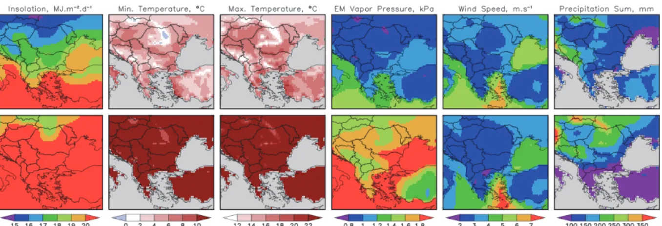
The WOFOST output includes the following time-depended variables: number of days since emergence, development stage of crop, thermal time since emergence, dry weight of living leaves, dry weight of living stems, dry weight of living storage organs, total above-ground production, leaf area index, transpiration rate, gross assimilation, maintenance respiration rate, and rate of dry matter increase. The process is repeated in a loop for every gridcell in the domain. Finally, the output aggregated for all gridcells is stored in external three-dimensional (in space and time) binary direct access file, which is a very convenient form of storage allowing additional post-processing with powerful instruments like GrADS. The meteorological data for the whole simulation period are also stored in such a file. This makes the further parallel analysis of the meteorological and crop-specific parameters possible. The seasonal average of the insolation, minimum temperature, maximum temperature, EM water vapor pressure, and wind speed ,as well as the precipitation sum for the spring (traditionally accepted as March, April, and May) and the summer (June, July and August), which are the two most relevant seasons to the crop development, are shown in Fig. 2.
Fig. 2. Seasonal averages of all meteorological parameters, except for precipitation as well as the precipitation sum for the spring (MAM, first row) and summer (JJA, second row).
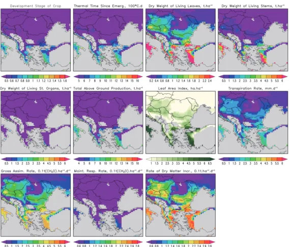
Figs. 3–6 show the spatial distributions of all 11 WOFOST-output parameters in approximately equidistant time intervals.
Fig. 3. Distribution of the WOFOST potential crop production output parameters on April 19.
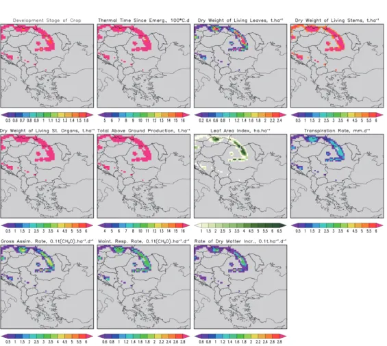
Fig. 4. Same as Fig. 3, but for May 29.
Fig. 5. Same as Fig. 3, but for July 8.
Fig. 6. Same as Fig. 3, but for August 17.
The obtained results can be generalized in many directions, but thus far, the main features of the achieved fields of the output variables seem evident. First, these fields are spatially and temporally consistent: the geographical distribution looks realistic, with well reproduced general north-south gradient, elevation, and coastal effects. The last two effects are especially discernible over the main Carpathian ridge and the northwestern coast of Turkey, correspondingly. The timeliness of the simulated crop calendar also seems realistic – the maximum of the dry weight of the storage organs, which is probably the most important parameter from practical point of view, is reached approximately, over the plains in the internal part of the domain, in the second half of June. The model system simulates also the time lag, i.e., the delay of the wheat development of the northern and elevated regions.
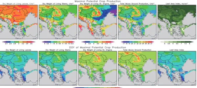
It is important, at least from practical point of view, to map the maximum value of, for reasons of brevity, only the 'yield-related' output variables and the day of the simulation (which in our case is equivalent to the day of the year (DOY)), when this maximum is reached. These maps are shown in Fig. 7.
Fig. 7. Maximum value of the yield-related WOFOST output variables and the day of the year, when this maximum is reached.
It is worth mentioning at least two peculiarities of the distributions of the maximums. First is the zone of low productivity, which is elongated from the northeastern corner of the domain to the center. This zone is most clearly expressed in the field of the maximum of dry weight of the storage organs. The reasons for appearance of this zone can be manifold, but most important is perhaps the reduced precipitation in the spring and summer over there, as shown in Fig. 2.
The second peculiarity seems at first slightly strange: the productivity over the semi-mountainous regions, which are traditionally not considered as suitable for crop breeding, is bigger than on the plains. This is especially good expressed in the foothill parts of the Carpathians. The plot of the time series of the WOFOST over two gridcells – the first over the Thracian valley in Bulgaria and the second over the Carpathians shows this clearly. In the first gridcell, the maximum is around the end of June and close to 8 t/ha, and in second cell is occurs almost a month later with values near 10 t/ha. In the first case, the main part of the crop development is in June and in the second – in July. Thus, probable explanations for the elevated winter wheat production in the second case are the more favorable weather conditions during the period of yields formation. More specially, the higher yields in more cooler regions are related to a longer growing period (and thus to a longer biomass accumulation period), and that there is a lower drought and heat stress frequency.
The DOY of the maximum of the considered variables and the interrelation between them also look realistic – the distribution of the DOY of the dry weight of leaving leaves and stems, as well as the DOY of the leaf area index are practically identical. The fields of the dry weight of the storage organs and total above-ground production are also identical. Most typical difference between the two groups is the time lag of approximately one month of the second in comparison with the first.
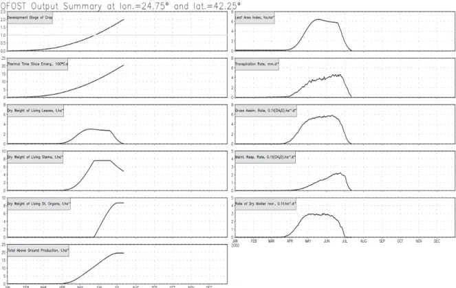
All of the described findings of the performed numerical simulation of the growth and development of winter wheat in Bulgaria and the Balkans, in particular, can be explained with physiological and biological lows of plant organisms. They go through two main stages of development – the vegetative and reproductive stages. During the vegetative stage of growth going on stems, leaves, and roots of the plants, the above descibed findings provide the necessary conditions for the formation and growth of reproductive organs that determines the size of yields. The leaves have the most important function until the moment of physiological maturation of plants. They are the photosynthetic apparatus that ensure the flow of assimilates for the whole plant. After flowering there is no increase of root activity and the root growth is dimishing (in cereals).
After formation of reproductive organs, function of leaves gradually decreases and the function of the stems increases that support the growth of these organs.
At the same time, a gradual yellowing and dying leaves upwards ensure the flow of assimilates only to the reproductive organs. The whole process is described by logistic or as it is known in biochemistry, autocatalytic functions. This fact justifies the differences in the dates for achieving maximum growth of aboveground parts of plants, as it is shown in Figs. 8–9.
Fig. 8. Time series of the WOFOST potential crop production output parameters for the gridcell in the Thracian valley.
Fig. 9. Same as Fig. 8, but for the gridcell in the Carpathian ridge.
4.Conclusion
The most significant outcome of the performed numerical experiment of the application of the crop model WOFOST in grid using meteorological input data from the reanalysis ERA-Interim and the objective analysis E-OBS is the spatial and temporal consistency of the produced output fields. Our study confirms the main conclusion in the work of de Wit et al., (2010) regarding the suitability of ERA-Interim for crop modelling. Although such results seem predictable, accounting, first, the spatial and temporal consistency of the input data and, second, the deterministic nature of the CP WOFOST, only the results of such successful simulation can proof this assumption with the necessary rigor. The main limitation of the model system is that only the potential crop production has been taken into consideration so far, which does not allow direct comparison with independent crop yield measurements, therefore, the outcome does not contradict basically with any empirically-derived agrometeorological principles.
The produced three-dimensional digital maps of the crop production related parameters offer possibilities of agrometeorological analysis, which would be impossible with the picture derived with meteorological data from limited number (and as rule randomly spread) of stations. Thus, in particular, interesting and significant facts about the spatial and temporal variation of the crop-specific parameters are revealed. The simulation outcome proofs the reliability and suitability of the datasets originated from RA and OA for crop modelling. This is a relevant step ahead in the authors’ general plan for preparing more detailed and realistic simulation system. The next step is to include more adequate soil inventory and crop calendar. Later, if implementing seasonal weather forecasting would allow running the system in forecast mode, a futher step will be to predict the future crop production related variables. Such information is of significant importance for wide range of experts and for scientific-based decision-making.
Acknowledgments: We acknowledge the E-OBS data-set from the EU-FP6 project ENSEMBLES (http://ensembles-eu.metoffice.com) and the data providers in the ECA&D project (http://www.ecad.eu). Deep gratitude to the ECMWF for the RA ERA-Interim, and to all other organizations and institutes (IGES/COLA, Unidata, MPI-M and all others) for providing free of charge software and data. Without their innovative data services and tools this study would be not possible. Personal thanks to Dr. Allard de Wit from WUR and Ivan Tzonevsky from ECMWF for the cooperation.
References
Boogaard, H.L., Van Diepen, C.A., Rötter, R.P., Cabrera, J.M.C.A. and Van Laar, H.H., 1998:
WOFOST 7.1 User’s guide for the WOFOST 7.1 crop growth simulation model and WOFOST Control Center 1.5. Technical Document 52 DLO Winand Staring Centre, Wageningen.
Dee, D.P., Uppala, S.M., Simmons, A.J., Berrisford, P., Poli, P., Kobayashi, S., Andrae, U., Balmaseda, M.A., Balsamo, G., Bauer, P., Bechtold, P., Beljaars, A.C.M., van de Berg, L., Bidlot, J., Bormann, N., Delsol, C., Dragani, R., Fuentes, M., Geer, A.J., Haimberger, L., Healy, S.B., Hersbach, H., Hólm, E. V., Isaksen, L., Kållberg, P., Köhler, M., Matricardi, M., McNally, A.P., Monge-Sanz, B. M., Morcrette, J.-J., Park, B.-K., Peubey, C., de Rosnay, P., Tavolato, C., Thépaut, J.-N. and Vitart, F., 2011: The ERA-Interim reanalysis: configuration and performance of the data assimilation system. Quart. J. Roy. Meteorol. Soc. 137, 553–597.
https://doi.org/10.1002/qj.828
Eitzinger, J., Thaler, S., Orlandini, S., Nejedlik, P., Kazandjiev, V., Håkon Sivertsen, T., and Mihailovic, D., 2009: Applications of agroclimatic indices and process oriented crop simulation models in European agriculture, Időjárás 113, 1–12.
Haylock, M.R., Hofstra, N., Klein Tank, A.M.G., Klok, E.J., Jones, P.D., and New, M., 2008: A European daily high-resolution gridded dataset of surface temperature and precipitation for 1950–2006, J. Geophys. Res. 113, D20119. https://doi.org/10.1029/2008JD010201
Kazandjiev V. and Georgieva, V., 2006: WOFOST Model Calibration for some Cereal Crops in Bulgaria. Proc. of 8th Conference on Meteorology – Climatology and Atmospheric Physics COMECAP 24-26 May 2006, Athens, ISBN 978-960-6806-01-8. 97–102.
Koynov, V., Kabakchiev, I., and Boneva, V., 1998: Атлас на почвите в България, Zemizdat, 321. (in Bulgarian)
Leo, O. and Baruth, B., 2013: MARS, the EU Crop monitoring and Yield Forecasting Systems proceeding of the SWF-GEOGLAM. International Meeting on Food Security, Earth Observations and Agricultural Monitoring November 21, 2013, Brussels available online at https://swfound.org/media/126467/10_rtd%20geoglam%20mars%2021%20oct%2013.pdf accessed on the 14.06.2017
Oteng-Darko, P., Yeboah, S., Addy, S.N.T., Amponsah S., and Owusu Danquah, E., 2013: Crop modelling: A tool for agricultural research – A review. E3 Journal of Agricultural Research and Development 2, 1–6, Available online http://www.e3journals.org
Rounsevell, M.D.A., Berry, P.M., and Harrison P.A., 2006: Future environmental change impacts on rural land usebiodiversity: a synthesis of the ACCELERATES project. Environ. sci. policy 9, 93–100. https://doi.org/10.1016/j.envsci.2005.11.001
de Wit, A.J.W., Baruth, B., Boogaard, H.L., van Diepen, C.A., van Kraalingen, D.W.G., Micale, F., te Roller, J.A., Supit, I., and van der Wijngaart, R., 2010: Using ERA-INTERIM for regional crop yield forecasting in Europe. Climate Res. 44, 41–53. https://doi.org/10.3354/cr00872