DOI:10.28974/idojaras.2018.3.3
IDŐJÁRÁS
Quarterly Journal of the Hungarian Meteorological Service Vol. 122, No. 3, July – September, 2018, pp. 259–283
Spatial analysis of air temperature and its impact on the sustainable development of mountain tourism in
Central and Western Serbia
Danijela Vukoičić1*, Saša Milosavljević1, Ivana Penjišević1, Nikola Bačević1, Milena Nikolić2, Radomir Ivanović1, and Bojana Jandžiković1
1 Department of Geography, Natural Sciences and Mathematics, University of Pristina, 38220 Kosovska Mitrovica, Serbia
2 Belgrade Business School, Higher Education Institution for Applied Studies, 11000 Belgrade, Serbia
*Corresponding author E-mail: danijela.vukoicic@pr.ac.rs (Manuscript received in final form May 29, 2017)
Abstract⎯Empirical studies of the late twentieth and early twenty-first century indicate the existence of a growth trend in air temperature. This trend is particularly pronounced in the region of Southern Europe, including the Republic of Serbia. Many problems occur in the socio-economic areas due to global warming, which directly influences the development of tourism. In this study, we will deal with the influence of climate change on the sustainable development of mountain tourism in the area of the western and central Serbia tourist zones, which includes Starovlaška and Kopaonik mountain chain. The data on changes in the temperature of air will be gathered at six different altitude meteorological stations, for the period from 1990 to 2014. All weather stations in the studied area were classified into three groups: lowland, middle and high mountain. In order to obtain trends, three sets of data were used: the average monthly temperature, the maximum monthly temperature, and the monthly minimum temperature, recorded in each station. The seasonal classification has been conducted based on four seasons: spring, summer, autumn, and winter. Three statistical approaches were used to analyze the temperature trends in 15 time series, for each group of stations individually. First, the trend equation was calculated for each time series, then, completely separate from the first approach, all trends were assessed using the Mann-Kendall test, and in the end, in all cases, the trend magnitude was calculated based on the trend equation. The results show that there is a significant positive trend of temperature rise on an annual basis, while the trend is significantly positive during the fall and spring seasons. In winter, the trend is slightly positive or absent, while in the summer trend is moderately positive in all three groups of stations.
Key-words: analysis of temperature, sustainable development, mountain tourism, turist zone, Serbia
1. Introduction
The analysis of the mean value of air temperature changes in the last couple of decades is an important theme of climate research. The studies include different regions in the world, and the scales show that there is an air temperature growth trend during the twentieth century (Jones and Moberg, 2003; Luterbacher et al., 2004; Rebetez and Reinhard, 2008; Manabe et al., 2011; Tabari and Talaee, 2011; Christy, 2013; Wang et al., 2014; Kuang et al., 2014; Omondi et al., 2014;
Croitoru et al., 2014). According to the Intergovernmental Panel on Climate Change report (IPCC, 2007), Europe is isolated as one of the regions especially sensitive to climate change. It is pointed out that climatic changes can increase regional differences concerning natural resources and their values. Mean annual temperatures in Europe in the last fifty years have increased faster than the global average. One of the regions where especially significant warming has been recorded is the southeast part of Europe. High temperatures can lead to a gradual decrease of summer tourism in the Mediterranean, but also to an increase in spring and autumn tourism. Ski resorts in Europe can be affected by a significant reduction in snow cover at the beginning and end of the winter season, which can significantly affect the overall economic development (Unger et al., 2016).
The Intergovernmental Panel on Climate Change report (IPCC, 2014) made a conclusion that the human impact on the climate is indisputable and that the effects can be seen in several regions of the world. High mountainous regions are the most exposed to big climate changes (Diaz and Bradley, 1997; Croitoru et al., 2014, 2016). The consequences of this are reflected in the different socio- economic and ecological areas: tourism industry, health of human population, ecosystems, mountain glaciers, water resources (Mountain Agenda, 1998;
Beniston, 2003, 2005; Walther et al., 2005; Boisvenue and Running, 2006; EEA, 2008; Micu, 2009, 2012; Toreti et al., 2010; Croitoru et al., 2014, 2016). There are a number of studies dealing with the analysis of climate change in Serbia.
Observed mean annual temperature in the last 50 years show a positive trend almost everywhere in Serbia. It is expected that the increase in temperature has a different trend during different seasons, up to 0.04 °C per year. The greatest increase in temperature is recorded during the fall period. The analysis of climate change through temperature trends was done on annual and seasonal levels for the whole territory of Serbia (Popović et al., 2005, 2009).
The individual linear trends were not measured for the stations in the mountainous areas of Serbia, neither were the impacts of climate change on tourism development in the region. The Republic of Serbia has a lot of potential for the development of mountain tourism, but only 30% are utilized (Milijić et al., 2013). These are high mountain areas above 1500 m above sea level (Kopaonik), and partly the medium height mountains, from 1000 to 1500 m high (Zlatibor, Tara, Zlatar). Given that previously performed studies of the highest
areas of Serbia (western and central tourist zones of Serbia) are modest and insufficient, the aim of this paper is to analyze temperature trends and highlight their impact on the sustainable development of mountain tourism.
2. Materials and methods 2.1. Area
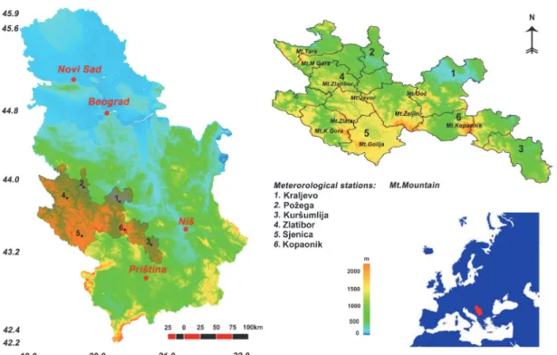
The research area is a mountainous area in Serbia that includes mountains of Starovlaška and Kopaonik, as well as part of a western zone under younger fold mountains. In structural terms, the western zone of younger fold mountains belong to the Dinaric Alps in the broad sense (Rodic and Pavlovic, 1994). It is part of the southern Alpine orogenic belt. It was formed during the late Alpine orogeny in a spacious geosyncline of Tethys. According to the geological structure, impervious Paleozoic rocks occupy the largest space, although Starovlaška mountains contain Mesozoic limestone as well. According to the spatial plan of the Republic of Serbia in 1996, the area of research belongs to the Western and Central Serbia tourist zone (Jovičić, 2009). In the regional organization of Serbian tourist area, Zlatibor tourist region (Tara-Zlatibor- Zlatar) belongs to the Western tourist zone, while Kopaonik and Golija belong to the Central tourist zone (Fig. 1).
Fig. 1. Western and Central Serbia tourist zone and spatial distribution of the analyzed meteorological stations on the Serbian map.
2.2. Data
This work contains an analysis of surface air temperature trends obtained for six meteorological stations. The locations of the stations are presented in Fig. 1, and their main parameters are given in Table 1 in accordance with the Hydrometeorological Service of Serbia (http://www.hidmet.gov.rs/). Weather stations are divided into three groups depending on the altitude of the area for the period (P) from 1990 to 2014. The western tourist zone has an altitude of 1500 m, the central tourist zone reaches 2017 m, and the valley areas of these zones range from 200 m to 500 m (Marović, 2001). Based on that, the cells are grouped into three groups: lowland (L), medium-sized mountains (M1), and high mountains (M2).
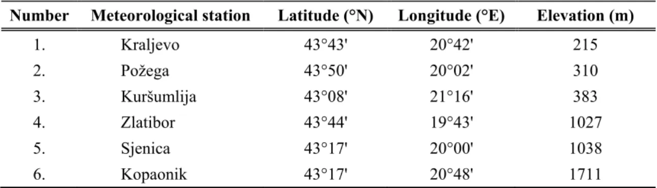
Table 1. List of meteorological stations and their geographical coordinates and elevations
Number Meteorological station Latitude (°N) Longitude (°E) Elevation (m)
1. Kraljevo 43°43' 20°42' 215
2. Požega 43°50' 20°02' 310
3. Kuršumlija 43°08' 21°16' 383
4. Zlatibor 43°44' 19°43' 1027
5. Sjenica 43°17' 20°00' 1038
6. Kopaonik 43°17' 20°48' 1711
In order to obtain trends, three sets of data were used: the average monthly temperature, the maximum monthly temperature, and the minimum monthly temperature for each station. Using the average monthly temperature, the minimum average annual temperature and the maximum average annual temperature have been calculated, as well as the average annual temperature and the average seasonal temperature for each season. Finally, based on these three types of average air temperature, new data sets for each month referred to as T, Tx, Tn are derived, for calculating trends for three lowland stations (L):
Kraljevo, Požega, and Kuršumlija; two stations in the medium-sized mountains (M1): Zlatibor and Sjenica, while Kopaonik was treated as a separate data set, because it is a high mountain station (M2).
Seasons definitions are used: winter (W), spring (Sp), summer (Su), and autumn (A), which are arranged in divided into sets of three months: January, February, and March; April, May, and June; July, August, and September; and October, November, and December (Hrnjak et al., 2014), respectively (Gavrilov et al., 2015).
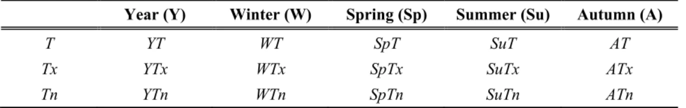
During this research, the database was formed according to the year (Y), season (W, Sp, Su, A), and three types of temperatures (T, Tx, and Tn). There are 15 stations in each group, 45 time series in total (15x3), which are used to determine the trend. Each of these 15 stations is marked with the acronym consisting of the abbreviation for the year/season and type of temperature (Table 2).
Table 2. List of 15 time series to calculate surface air temperature trends
Year (Y) Winter (W) Spring (Sp) Summer (Su) Autumn (A)
T YT WT SpT SuT AT Tx YTx WTx SpTx SuTx ATx Tn YTn WTn SpTn SuTn ATn
Before the previous calculation, the homogeneity of the temperature data was examined according to the Alexandersson (1986) test. The test showed that the time series are not non-homogeneous for a significance level of 5%
(Gavrilov et al., 2017).
2.3. Methodology
We adopted three statistical approaches in order to analyze the temperature trends in 15 time series, for each group of stations individually. First, we calculated the trend equation for each time series using linear interpolation of the mean annual and seasonal temperatures (Feidas et al., 2004). When the coefficient direction of the trend equation is greater than zero, the trend is positive, when it is less than zero, the trend is negative, and when it is equal to zero, there is no trend (no change). Completely independent of the first approach, in the second one we used the Mann-Kendall test (hereinafter MK test) in order to assess the significance of temperature trends (Kendall, 1938, 1975; Mann, 1945; Gilbert, 1987). This test is widely applicable in the climatological time series. Ultimately, the trend magnitude in all cases was calculated using the trend equation (Gavrilov et al., 2015, 2016, 2017).
According to the MK test, two hypotheses were tested: the null hypothesis, H0, when the trend is absent in the time series; and the alternative hypothesis, Ha, when there is a significant trend in the series, for a given level of significance. The probability, p, was calculated to determine the level of confidence in the hypothesis.
In the following study, the brief mathematical procedure for the hypothesis, test, and assessment of the significance of the temperature trends will be
described. A key step in the application of MK test is the calculation of the MK statistics (Karmeshu, 2012):
( )
1
1 1
sgn .
n n
j i
i j i
S − T T
= = +
=
− , (1)where:
( )
1 0sgn 0 0
1 0
j i
j i j i
j i
if T T
T T if T T
if T T
− >
− = − =
− − <
. (2)
Here, Tj and Ti are the time series of the annual and/or seasonal values of the temperatures in years j = i + 1, i + 2, i + 3,...,n and i = 1, 2, 3,..., n-1, where j
> i, and n is the last year in the time series.
As seen in Eqs. (1) and (2), if the temperature from the later year is higher than the temperature from the earlier year, S is incremented by 1. On the other hand, if the temperature from the later year is lower than the temperature of the earlier year, S is decremented by 1. The net result of all such increments and decrements yields the final value S. Statistics S can serve for evaluation of the temperature trend, because a very high positive value of S is an indicator of an increasing trend, and a very low negative value of S indicates a decreasing trend.
However, to statistically quantify the significance of the trend, it is necessary to compute the probability associated with S and the number of years, n.
Now, we will describe the procedure to compute this probability. For this purpose, the normalized/standard test statistic Z is calculated as:
1 0
0 0
1 0
S for S
Z for S
S for S
−
>
= =
+
<
σ σ
, (3)
where σ2 is the variance for the approximately normally distributed statistics S for n ≥ 10. Finally, for measuring the significance of the temperature trend, the probability p is computed as:
( )
1 100
p= − f Z ⋅ . (4)
Here, ƒ(Z), as the probability density function for a normal distribution with a mean of 0 and a standard deviation of 1, is given by the following equation:
( )
1 exp 222
f z Z
= −
π . (5)
As seen in Eq. (4), the probability p takes values between 0 and 100 in %.
In fact, p is used to test the level of confidence in the hypothesis (Gavrilov et al., 2010, 2011, 2013, 2015). If the computed value p is lower than the chosen significance level, α (e. g., α=5%), the H0 (there is no trend) should be rejected, and the Ha (there is a significant trend) should be accepted; and if p is greater than the significance level, the H0 cannot be rejected. We used XLSTAT software (http://www.xlstat.com/) for calculating the probability, p, and hypothesis testing.
It is considered that accepting the Ha indicates that a trend is statistically significant. On the other hand, acceptance of the H0 implies that there is no trend (no change), while often in practice, the trend equation indicates the opposite, i. e., there is a trend. Therefore, to reduce the contradiction in analyzing the temperature trends between two independent statistical approaches, trend equation, and applying the previous or classical interpretation of the MK test, the modified interpretation of the MK test will be used (Gavrilov et al., 2015).
It is quite clear that with decreasing the probability p, the statistical confidence in the H0 is decreasing and the confidence in the Ha is increasing, and vice versa. For the purposes of this study, a modified MK test with four levels of confidence was declared. Based on the computed probability p, these four levels of confidence are: less or equal than 5%: there is a significant positive/negative trend; greater than 5% and less or equal than 30%: there is a moderately positive/negative trend; greater than 30% and less or equal than 50%: there is a slightly positive/negative trend, and greater than 50%: there is no trend.
As it can be seen, in cases (a) and (d) both interpretations of the MK tests have the same meaning. Differences occur in cases (b) and (c), where the classical MK test claims there is no trend, and the modified MK test allows trend with reduced levels of confidence. It is clear that modified interpretation is more subtle, and it enables obtaining diverse assessments (Gavrilov et al., 2015).
Namely, the modified Mann–Kendall test is used for smoother quantization of confidence levels than the regular Mann-Kendall test. The Modified Mann–
Kendall test just verifies the results obtained by the direct method (for positive trend, the modified Mann-Kendall test shows positive moderate trend in cases when by observing Mann-Kendall tests no trend is detected because of more robust quantization of confidence level).
In the third statistical approach, the trend magnitude was calculated as:
(
1990) (
2014)
y y y
Δ = − , (6)
where Δy is the trend magnitude in °C, y (1990) and y (2014) are temperatures from the trend equation in the beginning, 1990, and at the end, 2014, of the period, both in °C. When Δy is greater than zero, less than zero, or equal to zero, the sign of the trend is negative (decrease), positive (increase), or no trend (no change), respectively. Moreover, when Δy is less than or equal to the standard error of the temperature measurement, certainly there is no trend (Gavrilov et al., 2015).
3. Results and discussion
Each of Figs. 4–12 shows annual and seasonal temperatures during the period 1990–2014, the trend equation, where y is the mean annual and seasonal value of the temperature in °C, x is the time in years; and the trend line. The probability confidence, p, and the trend magnitude, Δy, for each time series over the territory of the western and central tourist zones of Serbia are shown in Tables 4–6, respectively. In all cases, the significance level was the same, a=5%
(Karmeshu, 2012; Gavrilov et al., 2017).
Table 3. Probability confidences and trends magnitudes for all time series for the group of stations L
T Tx Tn p [%] Δy [°C] p [%] Δy [°C] p [%] Δy [°C]
Y 0.19 –1.35 2.23 –1.225 0.05 –1.4
W 42.72 –1.025 90.26 0.075 20.92 –1.55
Sp 3.43 –1.4 11.96 –1.475 1.72 –1.1
Su 4.97 –1.55 27.50 –1.475 4.40 –1.475
A 4.19 –1.1 6.27 –1.4 4.19 –1
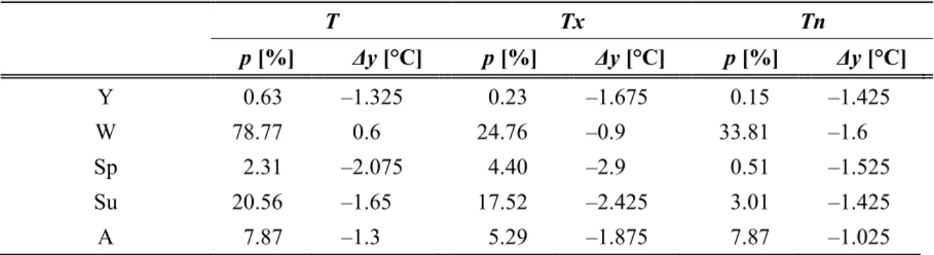
Table 4. Probability confidences and trends magnitudes for all time series for the group of stations M1
T Tx Tn p [%] Δy [°C] p [%] Δy [°C] p [%] Δy [°C]
Y 0.63 –1.325 0.23 –1.675 0.15 –1.425
W 78.77 0.6 24.76 –0.9 33.81 –1.6
Sp 2.31 –2.075 4.40 –2.9 0.51 –1.525
Su 20.56 –1.65 17.52 –2.425 3.01 –1.425
A 7.87 –1.3 5.29 –1.875 7.87 –1.025
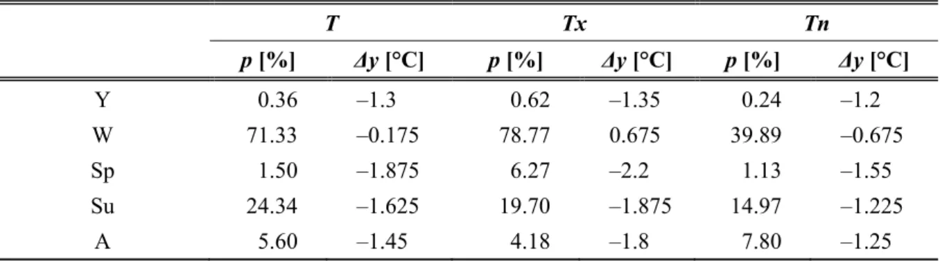
Table 5. Probability confidences and trends magnitudes for all time series for the group of stations M2
T Tx Tn p [%] Δy [°C] p [%] Δy [°C] p [%] Δy [°C]
Y 0.36 –1.3 0.62 –1.35 0.24 –1.2
W 71.33 –0.175 78.77 0.675 39.89 –0.675
Sp 1.50 –1.875 6.27 –2.2 1.13 –1.55
Su 24.34 –1.625 19.70 –1.875 14.97 –1.225
A 5.60 –1.45 4.18 –1.8 7.80 –1.25
Average maximum temperatures (Tx) in the area of the western and central tourist zones of Serbia for the period 1990–2014 are summarized in Fig. 2, which clearly indicates the observed temperature difference. In lowland areas (Kraljevo, Kuršumlija, and Požega), Tx ranges from 16.7 to 17.5 °C, in the middle-sized venues (Sjenica and Zlatibor) it is 13 °C, and in the higest mountainous areas (Kopaonik) Tx is 8 °C.
Fig. 2. Mean maximum air temperature (Tx) on an annual basis in the western and central tourist zones of Serbia for the period from 1990 to 2014.
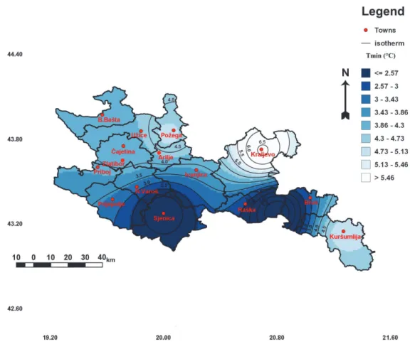
Fig. 3 shows the distribution average of minimum temperature (Tn). In the lowland areas of the western and central tourist zones, Tn ranges from 4.8 to 6.6 °C (Požega, Kraljevo, and Kuršumlija), and this difference is more pronounced in some areas of the middle-size mountain ranging from 1.5 °C (Sjenica) to 4.1 °C (Zlatibor). The highest mountain areas (Kopaonik) have an average minimum temperature (Tn) of 0.5 °C.
Fig. 3. Mean minimum air temperature (Tn) on an annual basis in the western and central tourist zones of Serbia for the period from 1990 to 2014.
In strictly formal terms, some trends can be observed in all cases. However, all trends do not have the same positive or negative sign, probability, and magnitude. In order to obtain a final evaluation of the temperature trends in the western and central tourist zones, all numerical parameters, the visual representation of trends and, most importantly, the results of both MK tests were used.
Figs. 4–6 and trend equations show that for the time series YT, WT, SpT, SuT, AT, YTx, SpTx, SuTx, ATx, YTn, WTn, SpTn, SuTn, and ATn, trends are positive; and in the cases of WTx, the trends are negative. MK testing will prove whether these statements are true.
(a) (b)
(c) (d)
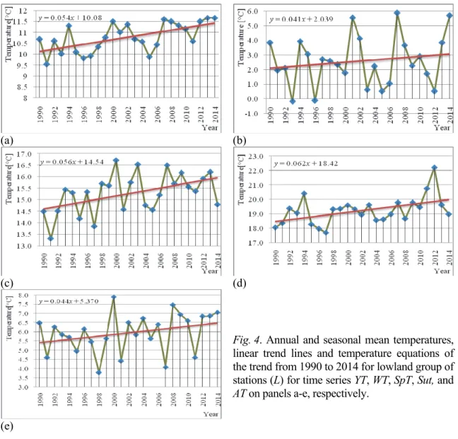
Fig. 4. Annual and seasonal mean temperatures, linear trend lines and temperature equations of the trend from 1990 to 2014 for lowland group of stations (L) for time series YT, WT, SpT, Sut, and AT on panels a-e, respectively.
(e)
Results shown in Fig. 4 and Table 3 where futher analyzed to estimate the final trends. As the computed values of probability p fot the time series YT, SpT, SuT and AT is lower than the level of significance of a=5%, the null hypothesis H0 should not reject, and alternative hypothesis Ha is accepted. The risks to reject the null hypothesis are smaller than 4.97% for all time series. The calculated p-value of the time series WT is greater than the level of significance of a=5%, so we can reject the null hypothesis H0. The risk to reject the null hypothesis H0 while it is true is 42.72%. In accordance with the classical MK tests, the first, third, fourth, and fifth cases have a positive trend, while the second case is without trend. The modified MK test declared that the first, third, fourth, and fifth cases have positive significant trend, while the second have slightly positive trend.
(a) (b)
(c) (d)
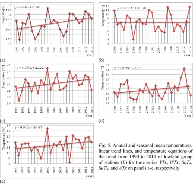
Fig. 5. Annual and seasonal mean temperatures, linear trend lines, and temperature equations of the trend from 1990 to 2014 of lowland group of stations (L) for time series YTx, WTx, SpTx, SuTx, and ATx on panels a-e, respectively.
(e)
Based on the observed results presented in Fig. 5 and Table 3, the hypothesis was futher analyzed. Since the calculated value of p of the time series YTx is lower than the level of significance a=5%, the null hypothesis H0 should be reject, and the alternative hypothesis Ha is accepted. The risk to reject the null hypothesis is less than 2.23%. The calculated p value of the time series WTx, SpTx, SuTx and ATx are higher than the level of significance of a=5%, so it can not reject the null hypothesis H0. The risk to reject the null hypothesis H0 while it is true is 90.26, 11.96, 27.50, and 6.27 (all in %) for all time series, respectively. In accordance with the classical MK tests, the second, third, fourth, and fifth cases are without trend, while the first case has a trend. The modified MK test declared that the third, fourth and fifth cases have moderately positive trend, the first has positive significant trend, while the second case is without trend.
(a) (b)
(c) (d)
Fig. 6. Annual and seasonal mean temperatures, linear trend lines, and temperature equation of the trend from 1990 to 2014 for lowland group of stations (L) for time series YTn, WTn, SpTn, SuTn, and ATn on panels a-e, respectively.
(e)
Fig. 6 and Table 3 give the values of the analyzed hypothesis. Since the calculated p value of the time series YTn, SpTn, SuTn, and ATn is lower than the significance level a=5%, we should reject the null hypothesis H0 and accept the alternative hypothesis Ha. Risks to reject the null hypothesis are less than 4.40%
for all time series. The calculated p value of the time series WTn is greater than the level of significance of a=5%, so we can reject the null hypothesis H0. The risk to reject the null hypothesis H0 while it is true is 20.92%. In accordance with the classical MK tests, the first, third, fourth, and fifth cases have a trend, while the second case is without trend. The modified MK test declared that the first, third, fourth, and fifth cases have positive significant trend, while the second case has moderately positive trend.
Figs. 7–9 and trend equations show that for the time series YT, SpT, SuT, AT, YTx, WTx, SpTx, SuTx, ATx, YTn, WTn, SpTn, SuTn, and ATn trends are positive; and in the WT cases the trends are negative. MK testing will prove whether these statements are true.
(a) (b)
(c) (d)
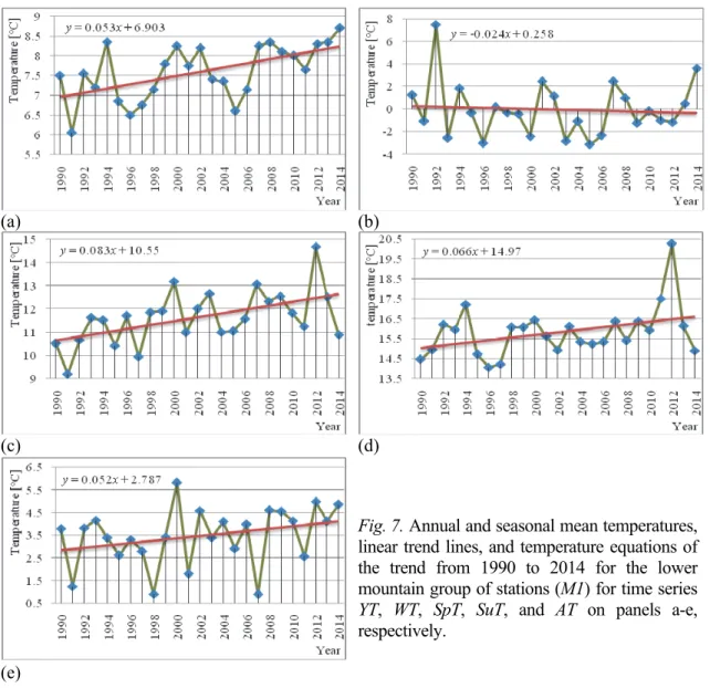
Fig. 7. Annual and seasonal mean temperatures, linear trend lines, and temperature equations of the trend from 1990 to 2014 for the lower mountain group of stations (M1) for time series YT, WT, SpT, SuT, and AT on panels a-e, respectively.
(e)
Results of the mean annual and seasonal temperature for the lower mountain group of station (M1) are shown in Fig. 7 and Table 4. The calculated p value of the time series YT and SpT is lower than the level of significance of a=5%, so we can reject the null hypothesis H0 and to accept the alternative hypothesis Ha. The risk to reject the null hypothesis is lower than 2.31% in both series. The calculated p value of the time series WT, SuT and AT is greater than the level significance of a=5%, so we can reject the null hypothesis H0. The risks to reject the null hypothesis while it is true are 78.77, 20.56, and 7.87 (all in %) for all time series, respectively. In accordance with the classical MK tests, the first and third cases have a trend, the second, fourth, and fifth cases are without trend. The modified MK test declared that the first and third case have positive significant trend, the fourth and fifth cases have moderately positive trend, while the second case is without trend.
(a) (b)
(c) (d)
Fig. 8. Annual and seasonal mean temperatures, linear trend lines, and temperature equation of the trend from 1990 to 2014 for the lower mountain group of stations (M1) for time series YTx, WTx, SpTx, SuTx, and ATx on panels a-e, respectively.
(e)
Fig. 8 and Table 4 give the results of the analyzed hypotheses. As the computed values of probability p for the time series WTx, SuTx and ATx are greater than the significance level a=5%, the H0 cannot be rejected in all cases.
The risks to reject the null hypothesis while it is true are 24.76, 17.52, and 5.29 (all in %) for all time series, respectively. In accordance with the classical MK tests, the second, fourth, and fifth cases are without trend. The modified MK test declared that all cases have moderately positive trend.
As the computed probability value p for the time series YTx and SpTx are lower than the significance level a=5%, the H0 should be rejected, and the Ha should be accepted for both time series. The risks to reject the null hypothesis are lower than 4.40%. The statement that there is a significant trend is correct with probabilities greater than 95.60% in both MK tests.
(a) (b)
(c) (d)
Fig. 9. Annual and seasonal mean temperatures, linear trend lines and temperature equations of the trend from 1990 to 2014 for the lower mountain group of stations (M1) for time series YTn, WTn, SpTn, SuTn, and ATn on panels a-e, respectively.
(e)
Fig. 9 and Table 4 show the results which were further analyzed. As the computed values of probability p for the time series WTn and ATn are greater than the significance level a=5%, the H0 cannot be rejected in all cases. The risks to reject the null hypothesis while it is true are 33.81 and 7.87%. In accordance with the classical MK tests, the second and fifth cases are without trend, while the modified MK test declared that second case has slightly positive trend, and the fifth case has moderately positive trend.
As the computed probability p value for the time series YTn, SpTn, and SuTn are lower than the significance level a=5%, the H0 should be rejected and the Ha should be accepted for both time series. The risks to reject the null hypothesis are lower than 3.01%. The statement that there is a significant trend is correct with probabilities greater than 96.99% in both MK tests.
Figs. 10–12 and trend equations show that for the time series YT, WT, SpT, SuT, AT, YTx, SpTx, SuTx, ATx, YTn, WTn, SpTn, SuTn and ATn trends are positive; and in the case WTx, the trend is negative. MK testing will prove whether these statements are true.
(a) (b)
(c) (d)
Fig. 10. Annual and seasonal mean temperatures, linear trend lines, and temperature equations of the trend from 1990 to 2014 for the high mountain group of stations (M2) for time series YT, WT, SpT, SuT, and AT on panels a-e, respectively.
(e)
Results of the mean annual and seasonal air temperature for the high mountainous group of stations (M2) are shown in Fig. 10 and Table 5. As the computed values of probability p for the time series WT, SuT, and AT are greater than the significance level α=5%, the H0 cannot be rejected in all cases. The risks to reject the null hypothesis when it is true are 71.33, 24.34, and 5.60 (all in %) for all time series, respectively. In accordance with the classical MK tests, it can be declared that there was no trend in all cases, while the modified MK test declared that the second case has no trend, and the fourth and fifth cases have moderately positive trend.
As the computed probability value p for the time series YT and SpT are lower than the significance level a, the H0 should be rejected and the Ha should be accepted for both time series. The risks to reject the null hypothesis are lower than 1.50%. The statement that there is a significant trend is correct with probabilities greater than 98.50% in both MK tests.
(a) (b)
(c) (d)
Fig. 11. Annual and seasonal mean temperatures, linear trend lines, and temperature equations of the trend from 1990 to 2014 for the high mountain group of stations (M2) for time series YTx, WTx, SpTx, SuTx, and ATx on panels a-e, respectively.
(e)
Fig. 11 and Table 5 show the results of the hypotheses, which were futher analyzed for the final assessment of trends in air temperature. As the computed values of probability p for the time series WTx, SpTx, and SuTx are greater than the significance level a=5%, the H0 cannot be rejected in all cases. The risks to reject the null hypothesis while it is true are 78.77, 6.27, and 19.70 (all in %) for all time series, respectively. In accordance with the classical MK tests, the second, third and fourth case are without trend, while the modified MK test declared that third and fourth case have moderately positive trend, and second case have no trend.
As the computed probability value p for the time series YTx and ATx are lower than the significance level a, the H0 should be rejected, and the Ha should be accepted for both time series. The risks to reject the null hypothesis are lower than 4.18%. The statement that there is a significant trend is correct with probabilities greater than 95.82% in both MK tests.
(a) (b)
(c) (d)
Fig. 12. Mean values of annual and seasonal temperature, linear trend line and temperature equation of trend from 1990 to 2014 for the high mountain group of stations (M2) for time series YTn, WTn, SpTn, SuTn, and ATn on panels a-e, respectively.
(e)
Results of the analyzed hypothesis (Fig. 12 and Table 5) were futher analyzed in order to obtain the final temperature trend estimates. As the computed values of probability p for the time series WTn, SuTn and ATn are greater than the significance level α=5%, the H0 cannot be rejected in all cases. The risks to reject the null hypothesis when it is true are 39.89, 14.97, and 7.80 (all in %) for all time series, respectively. In accordance with the classical MK tests, the second, fourth, and fifth cases are without trend, while the modified MK test declared that the fourth and fifth cases have moderately positive trend and the second case has slightly positive trend.
As the computed probability value p for the time series YTn and SpTn are lower than the significance level a, the H0 should be rejected, and the Ha should be accepted for both time series. The risks to reject the null hypothesis are lower than 1.13%. The statement that there is a significant trend is correct with probabilities greater than 98.87% in both MK tests.
The main results of our analysis of temperature trends in the western and central tourist zones in Serbia are given in Tables 6–8 depending on the altitude of the hydrometeorological stations. It seems that the positive temperature trends are dominant.
Table 6. The main results of the analysis of temperature trends for the lowland group of stations (L)
Time series Trend equation Classical MK test Modified MK test YT positive trend positive significant trend positive significant trend
WT positive trend no trend slightly positive trend
SpT positive trend positive significant trend positive significant trend SuT positive trend positive significant trend positive significant trend AT positive trend positive significant trend positive significant trend YTx positive trend positive significant trend positive significant trend
WTx negative trend no trend no trend
SpTx positive trend no trend positive moderate trend
SuTx positive trend no trend positive moderate trend
ATx positive trend no trend positive moderate trend
YTn positive trend positive significant trend positive significant trend
WTn positive trend no trend positive moderate trend
SpTn positive trend positive significant trend positive significant trend SuTn positive trend positive significant trend positive significant trend ATn positive trend positive significant trend positive significant trend
In accordance with the trend equations in the lowland group of stations (L), positive trends were found in 14 time series and negative trends were found only in one of them. After applying the classical MK test, only nine positive trends were statistically significant, and in the remaining cases there were no trends.
Also, after applying the modified MK test, (I) significant positive trends were confirmed in nine time series; and in the remaining cases the trends were declared as: (II) moderately and slightly positive in four series; (III) moderately and slightly negative in one case; and (IV) there was no trend in one case.
For all temperatures, T, Tx, and Tn, the annual trends were declared as significantly positive. All winter trends were declared as significantly positive, moderately positive and without a trend. The spring, summer, and autumn trends were declared as significantly positive, moderately positive, and significantly positive, respectively.
In accordance with the trend equations for the lower mountain group of stations (M1), positive trends were found in 14 time series, and negative trends were found only in one of them. After applying the classical MK test, only seven positive trends were statistically significant, and in the remaining cases there were no trends. Also, after applying the modified MK test, (I) significant positive trends were confirmed in seven time series; and in the remaining cases the trends were declared as: (II) moderately and slightly positive in six series;
(III) moderately and slightly negative in one case; and (IV) there was no trend in one case.
Table 7. The main results of the analysis of temperature trends for the lower mountain group of stations (M1)
Time series Trend equation Classical MK test Modified MK test YT positive trend positive significant trend positive significant trend
WT negative trend no trend no trend
SpT positive trend positive significant trend positive significant trend
SuT positive trend no trend positive moderate trend
AT positive trend no trend positive moderate trend
YTx positive trend positive significant trend positive significant trend
WTx positive trend no trend positive moderate trend
SpTx positive trend positive significant trend positive significant trend
SuTx positive trend no trend positive moderate trend
ATx positive trend no trend positive moderate trend
YTn positive trend positive significant trend positive significant trend
WTn positive trend no trend slightly positive trend
SpTn positive trend positive significant trend positive significant trend SuTn positive trend positive significant trend positive significant trend
ATn positive trend no trend positive moderate trend
For all temperatures, T, Tx, and Tn, the annual trends were declared as significantly positive. All winter trends were declared nonexistent, moderately positive, and slightly positive. All spring trends were declared significantly positive. Summer trends are declared as moderately positive and significantly positive, while the autumn trends were moderately positive.
Table 8. The main results of the analysis of temperature trends for the high mountain group of stations (M2)
Time series Trend equation Classical MK test Modified MK test YT positive trend positive significant trend positive significant trend
WT positive trend no trend no trend
SpT positive trend positive significant trend positive significant trend
SuT positive trend no trend positive moderate trend
AT positive trend no trend positive moderate trend
YTx positive trend positive significant trend positive significant trend
WTx negative trend no trend no trend
SpTx positive trend no trend positive moderate trend SuTx positive trend no trend positive moderate trend ATx positive trend positive significant trend positive significant trend YTn positive trend positive significant trend positive significant trend
WTn positive trend no trend slightly positive trend
SpTn positive trend positive significant trend positive significant trend SuTn positive trend no trend positive moderate trend
ATn positive trend no trend positive moderate trend
In accordance with the trend equations for the high mountain group of stations (M2), positive trends were found in 14 time series and negative trends were found in one time series. After applying the classical MK test, only 6 positive trends were statistically significant, and in the remaining cases there were no trends. Also, after applying the modified MK test, (I) significant positive trends were confirmed in 6 time series; and in the remaining cases the trends were declared as: (II) moderately and slightly positive in six series; (III) moderately and slightly negative in one case; and (IV) in two cases trend was nonexistent.
For all temperatures, T, Tx, and Tn, the annual trends were declared as significantly positive. With winter trends, in two cases there was no trend, and in the third case the trend was slightly positive. For the spring, trends were found significantly positive, moderately positive, and significantly positive. As for summer, trends are declared as moderately positive, while the autumn trends were moderately positive and significantly positive.
The results show that there is a significant positive trend of temperature rise on an annual basis, while the trend is significantly positive during the autumn and spring seasons. In winter, the trend is slightly positive or absent, while in summer the trend is moderately positive in all three groups of stations.
4. Conclusions
In the researched area, the mountain tourism takes place in the areas over 1000 m above sea level, so that climate changes directly affect areas of the western tourist zone and the lower parts of the central zone (from 1000 to 1500 m above sea level).
Thus, this area, as a future development factor, represents a new subject of planning for the protection and sustainable development. The new strategies have to be based on the experiences of the countries with a higher level of development of mountain areas, on the examples of tourism development. Research has proven that there is no trend int he average temperatures on an annual basis in the winter for middle-sized mountain areas, up to 1500 m above sea level, and that the trend int he mean maximum temperature on an annual basis is moderately positive, while the average minimum temperature recorded a slight growth.
In other seasons, there is a significantly positive and moderately positive temperature trend, which gives priority to the development of summer tourism.
The traditional way of doing agriculture and the arrangement of traditional settlements in this area are complementary to other activities. Protection and presentation of nature and natural values of these areas in the future give priority to the development of health and recreational tourism (Zlatibor, Zlatar, Tara, Brzeće).
Medium high and high mountain areas (Kopaonik), which were explored here, were equally affected by the current climate changes, while the consequences for mountain tourism were significant in lower areas. This impact will vary with the increasing altitude, and a small increase in winter temperatures can eliminate ski-centers at lower altitudes. Thus, the importance of high-mountain tourist centers and the need for sustainable development is increased.
References
Alexandersson, H., 1986: A homogeneity test applied to precipitation data. J. Climatol. 6, 661–675.
https://doi.org/10.1002/joc.3370060607
Beniston, M., 2005: Mountain climates and climatic change: An overview of processes focusing on the European Alps. Pure Appl. Geophys. 162, 8–9. https://doi.org/10.1007/s00024-005-2684-9 Beniston, M., 2003: Climatic change in mountain regions: a review of possible impacts. Climatic
Change 59, 5–31. https://doi.org/10.1023/A:1024458411589
Boisvenue, C. and Running, S.W., 2006: Impacts of climate change on natural forest productivity — evidence since the middle of the 20th century. Glob. Change Biol. 12, 862–882.
https://doi.org/10.1111/j.1365-2486.2006.01134.x
Christy, J.R., 2013: Monthly temperature observations for Uganda. J. Appl. Meteorol. Climatol. 52, 2363–2372. https://doi.org/10.1175/JAMC-D-13-012.1
Croitoru, A.E., Drignei, D., Dragotă, C.S., Imecs, Z., and Burada, D.C., 2014: Sharper detection of winter temperature changes in the Romanian higher-elevations. Glob. Planet. Change 122, 122–129.
https://doi.org/10.1016/j.gloplacha.2014.08.011
Croitoru, A.E., Drignei, D., Burada, D.C., Dragota, C.S., and Imecs, Z., 2016: Altitudinal changes of summer air temperature trends in the Romanian Carpathians based on serially correlated models. Quaternary Int. 415, 336–343. https://doi.org/10.1016/j.quaint.2015.05.075
Diaz, H.F. and Bradley, R.S., 1997: Temperature variations during the last century at high elevation sites. Climatic Change 36, 253–279. https://doi.org/10.1023/A:1005335731187
EEA, 2008: Impacts of Europe's Changing Climate – 2008 Indicator Based Assessment, EEA Report 4.
Feidas, H., Makrogiannis, T., and Bora-Senta, E., 2004: Trend Analysis of Air Temperature Time Series in Greece and their Relationship with Circulation Using Surface and Satellite Data: 1955- 2001, Theor. Appl. Climatol. 79, 185-208. https://doi.org/10.1007/s00704-004-0064-5
Gavrilov, M.B., Lazić, L., Pešić, A., Milutinović, M., Marković, D., Stanković, A. and Gavrilov, M., 2010:
Influence of hail suppression on the hail trend in Serbia. Physical geography 31(5): 441–454.
https://doi.org/10.2747/0272-3646.31.5.441
Gavrilov, M.B., Lazić, L., Milutinović, M., and Gavrilov, M.M., 2011: Influence of hail suppression on the hail trend in Vojvodina, Serbia. Geographica Pannonica 15, 36–41.
https://doi.org/10.5937/GeoPan1102036G
Gavrilov, M.B., Marković, S.B., Zorn, M., Komac, B., Lukić, T., Milošević, M., and Janićević, S., 2013:
Is hail suppression useful in Serbia? – General review and new results. Acta Geographica Slovenica 53, 165–179. https://doi.org/10.3986/AGS53302
Gavrilov, M.B., Marković, S.B., Jarad, A., and Korać, V.M., 2015: The analysis of temperature trends in Vojvodina (Serbia) from 1949 to 2006. Thermal Sci. 19, 339–350.
https://doi.org/10.2298/TSCI150207062G
Gavrilov, M.B., Tošić, I., and Marković, S.B., 2016: The analysis of annual and seasonal temperature trends using the Mann-Kendall test in Vojvodina, Serbia. Időjárás 120, 183–198.
Gavrilov, M.B., Marković, S.B., Janc, N., Nikolić, M., Valjarević, A.Đ., Komac, B., Zorn, M., Punišić, M., and Bačević, N., 2017: Assessing average annual air temperature trends using the Mann- Kendall test in Kosovo. Acta Geographica Slovenica 58, 7–26.
https://doi.org/10.3986/AGS.1309
Gilbert, R.O., 1987: Statistical Methods for Environmental Pollution Monitoring. Wiley, New York, USA
Hrnjak, I., Lukić, T., Gavrilov, M.B., Marković, S., Unkašević, M., and Tošić I., 2014: Aridity in Vojvodina, Serbia. Theor. Appl. Climatol. 115, 323–332.
https://doi.org/10.1007/s00704-013-0893-1
IPCC, 2007: Climate Change 2007: Synthesis Report. Contribution of Working Groups I, II and III to the Fourth Assessment Report of the Intergovernmental Panel on Climate Change [Core Writing Team, Pachauri, R.K and Reisinger, A. (eds.)]. IPCC, Geneva, Switzerland.
IPCC, 2014: Climate Change 2014: Synthesis Report. Contribution of Working Groups I, II and III to the Fifth Assessment Report of the Intergovernmental Panel on Climate Change [Core Writing Team, R.K. Pachauri and L.A. Meyer (eds.)]. IPCC, Geneva, Switzerland.
Jones, P.D. and Moberg, A., 2003; Hemispheric and Large-Scale Surface Air Temperature Variations:
An Extensive Revision and Update to 2001. Journal of Climate, 16, 206-223.
Jovičić, D., 2009: Turistička geografija Srbije. Univerzitet u Beogradu, Geografski fakultet, Beograd.
Karmeshu, N., 2012: Trend Detection in Annual Temperature & Precipitation using the Mann Kendall Test – A Case Study to Assess Climate Change on Select States in the Northeastern United States. M. Sc. thesis, University of Pennsylvania. USA.
Kendal, M., 1938: A new measure of rank correlation. Biometrica 30, 81–89.
https://doi.org/10.1093/biomet/30.1-2.81
Kendall, M.G., 1975; Rank correlation methods, 4th end. Charles Griffin, London.
Kuang, X.Y., Zhang, Y.C., Huang, Y., and Huang, D.Q., 2014: Changes in the frequencies of record- breaking temperature events in China and its association with East Asian Winter Monsoon variability. J. Geophys. Res. Atmos. 119, 1234–1248. https://doi.org/10.1002/2013JD020965 Luterbacher, J., Dietrich, D., Xoplaki, E., Grosjean, M., and Wanner, H., 2004: European seasonal and
annual temperature variability, trends and extremes since 1500. Science 303 (5663): 1499- 503.
Mann, H.B., 1945: Non-parametric tests against trend. Econometrica 13, 245–259.
https://doi.org/10.2307/1907187
Manabe, S., Ploshay, J., and Lau, N.C., 2011: Seasonal variation of surface temperature change during the last several decades. J. Climatol. 24, 3817–3821. https://doi.org/10.1007/s00703-009-0035-6 Marović, M., 2001: Geologija Jugoslavije. Rudarsko–geološki fakultet Univerzitet u Beogradu,
Beograd. (in Serbian)
Micu, D., 2009: Snow pack in the Romanian Carpathians under changing climatic conditions.
Meteorol. Atmosp. Phys.105, 1–16. https://doi.org/10.1007/s00703-009-0035-6
Micu, D., 2012: Cold waves in the Romanian Carpathians, an indicator of negative temperature extremes. Proceedings of the Conference Air and Water - Components of the Environment, IV.
Cluj University. 97–104.
Milijić, S., and Nenković-Riznić, M. 2013: Sustainable development of mountain areas – planning and protection in the context of climate change. Climate change and the built environment policies and practice in Scotland and Serbia. Monography, Special edition 70, 137–164.
Mountain Agend, 1998: Mountains of the World: Waters Towers for the 21st Century, Prepared for the United Nations Commission on Sustainable Development Institute of Geography, University of Berne (Centre for Development and Environment and Group for Hydrology) and Swiss Agency for Development and Cooperation Paul Haupt, Bern, Switzerland.
Omondi, P.A., Awange, J.L., Forootan, E., Ogallo, L.A., Barakiza, R., Girmaw,G.B., Fesseha, I., Kululetera, V., Kilembe, C., Mbati, M.M., Kilavi, M., King'uyu, S.M., Omeny, P.A., Njogu, A., Badr, E.M., Musa, T.A., Muchiri, P., Bamanya, D., and Komutunga, E., 2014. Changes in temperature and precipitation extremes over the Greater Horn of Africa region from 1961 to 2010. Int. J. Climatol. 34, 1262–1277. https://doi.org/10.1002/joc.3763
Popovic, T., Radulovic, E., and Jovanovic, M., 2005: Koliko nam se menja klima, kakva ce biti nasa buduca klima? In: EnE05—Zivotna sredina ka Evropi, Beograd. 210–218. (In Serbian)
Popovic, T., Djurdjevic, V., Zivkovic, M., Jović, B., and Jovanović, M., 2009: Promena klime u Srbiji i očekivani uticaji. Ministarstvo zastite zivotne sredine, Agencija za zastitu zivotne sredine Republike Srbije, Peta regionalna konferencija “EnE09—Zivotna sredina ka Evropi”. (In Serbian) www.sepa.gov.rs (In Serbian)
Republic Hydromet. Service of Serbia,
http://www.hidmet.gov.rs/ciril/meteorologija/klimatologija_godisnjaci.php
Rebetez, M., and Reinhard, M., 2008: Monthly air temperature trends in Switzerland 1901-2000 and 1975-2004.Theor. Appl. Climatol. 91, 27-34. DOI 10.1007 / s00704-007-0296-2
Rodić, D. and Pavlović, M., 1994; Zapadna zona mlađih venačnih planina i kotlina. U: Geografija Jugoslavije. Savremena administracija, Beograd. 62–73. (In Serbian)
Tabari, H. and Talaee, P.H., 2011: Analysis of trends in temperature data in arid and semi-arid regions of Iran. Glob. Planet. Change 79, 1–10. https://doi.org/10.1016/j.gloplacha.2011.07.008
Toreti, A., Desiato, F., Fioravanti, G., and Perconti, W., 2010: Seasonal temperatures over Italy and their relationship with low-frequency atmospheric circulation patterns. Climatic Change 99, 211–227. https://doi.org/10.1007/s10584-009-9640-0
Unger, R., Abegg, B., Mailer, M., and Stampfl, P., 2016: Energy Consumption and Greenhouse Gas Emissions Resulting From Tourism Travel in an Alpine Setting. Mount. Res. Develop. 36, 475–483.
https://doi.org/10.1659/MRD-JOURNAL-D-16-00058.1
Walther, G.R., Beissner, S., and Burga, C.A., 2005: Trends in upward shift of alpine plants. Journal of Vegetation Science 16: 541–548. www.meteoromania.ro (accessed 04. 28.15.)
Wang, S.J., Zhang, M.J., Pepin, N.C., Li, Z., Sun, M., Huang, X. and Wang, Q., 2014: Recent changes in freezing level heights in High Asia and their impact on glacier changes. J. Geophys. Res.
Atmos. 119, 1753–1765.https://doi.org/10.1002/2013JD020490 XLSTAT, http://www.xlstat.com/en/ (accessed 5.12.2016)