IDŐJÁRÁS Quarterly Journal of the Hungarian Meteorological Service

DOI:10.28974/idojaras.2018.3.1

IDŐJÁRÁS

Quarterly Journal of the Hungarian Meteorological Service Vol. 122, No. 3, July – September, 2018, pp. 217–235

The analysis of climatic indicators using different growing season calculation methods – an application to grapevine

grown in Hungary

Ildikó Mesterházy¹*, Róbert Mészáros², Rita Pongrácz^2,3, Péter Bodor⁴, and Márta Ladányi¹

1Department of Biometrics and Agricultural Informatics, Szent István University, Villányi út 29-43., H-1118 Budapest, Hungary

2Department of Meteorology, Eötvös Loránd University, Pázmány P. sétány 1/A, H-1117 Budapest, Hungary

3Excellence Center, Faculty of Science, Eötvös Loránd University, Brunszvik u. 2., H-2462 Martonvásár, Hungary

4Department of Viticulture, Szent István University, Villányi út 29-43., H-1118 Budapest, Hungary

*Corresponding author E-mail: Mesterhazy.Ildiko@kertk.szie.hu (Manuscript received in final form August 8, 2017)

Abstract―The precise knowledge of the beginning and the end of the growing season is necessary for the calculation of climatic indicators with evident effect on grapevine production. The aim of this study is to develop suitable methods on the basis of thermal conditions that can be used for calculation of the beginning, the end, and the length of the growing season for every single year. The two most accurate methods (‘5mid’ and ‘int’) are selected using the root-mean-square error compared to the reference growing season values based on averaging the daily mean temperature for several decades. In case of the

‘5mid’ method, the beginning (or the end) is the middle day of the first (or last) 5-day period with temperature not less than 10 °C. In case of the ‘int’ method, the beginning (or the end) of the growing season is the day after March 15 (or September 15), when the smoothed series of daily temperature using the monthly average temperatures of March and April (or September and October) exceeds 10 °C (or falls below 10 °C). As a next step, several climatic indicators (e.g., Huglin index and hydrothermal coefficient) are calculated for Hungary for three time periods (1961−1990, 2021−2050, and 2071−2100*) using the

‘5mid’ and ‘int’ methods. For this purpose, the bias-corrected daily mean, minimum, and maximum temperature and daily precipitation outputs of three different regional climate models (RegCM, ALADIN, and PRECIS) are used. Extreme temperature and precipitation

* In the case of the PRECIS model, due to its shorter simulation time range, we calculated the indicators for the period 2069−2098.

indices are also evaluated as they determine the risk of grapevine production. The spatial distributions of the indicators are presented on maps. We compare the indicators for the past and for the future using one-way completely randomized robust ANOVA (analysis of variance).

Results suggest that changes of temperature conditions in the 21st century will favor the production of red grapevine and late-ripening cultivars. Furthermore, drought seasons will be longer and extreme high summer temperatures will become more frequent, which are clearly considered as high risk factors in grapevine production. Besides the negative effects, the risk of winter frost damage is expected to decrease, which is evidently a favorable change in terms of grapevine production.

Key-words: Vitis vinifera, growing season calculation method, climatic indicator, ANOVA, Bonferroni’s correction, RegCM, ALADIN, PRECIS

1. Introduction

Grapevine production in Hungary is enabled by favorable climatic conditions.

Certain climatic events, however, can result in risk factors to the current production practices including the selection of specific grapevine cultivars. In this study, we apply indicators related to risk factors, and analyze their temporal and spatial changes.

Wine regions can be characterized with climate indicators that have evident effect on grapevine production based on temperature and precipitation (Hlaszny, 2012; Ramos et al., 2008; Santos et al., 2012). The comparison of vine growing regions worldwide can be done by analyzing the climate indicators based on observed meteorological data (Bois et al., 2012; Jones et al., 2009). These indicators can also be calculated using climate model simulation outputs for the 21st century (Hlaszny, 2012; Moriondo et al., 2013; Neumann and Matzarakis, 2011; Szenteleki et al., 2012). These results predict the changes in risk factors (e.g., long dry period and extreme heat), thus they can help farmers make long term decisions about the selection of favorable grapevine cultivars. Usually, a fixed growing season time interval is used in the calculation of the indicators, although the beginning and the end of the growing season depend on the actual meteorological conditions of each year. Since the variability of meteorological parameters (especially temperature) is expected to increase during the 21st century (IPCC, 2013), a modified growing season calculation method is reasonable to be used. It is desirable to find methods, which can handle the increasing frequency of extreme meteorological events.

Instead of the commonly used fixed time interval definition (i.e., April 1 – September 30), we calculate the length of the growing season on the basis of actual thermal conditions with the ultimate aim to develop suitable methods for determining the beginning, the end, and the length of the growing season by taking into account the different meteorological conditions throughout every single year.

The methods introduced in this study can handle the extreme temperature events of each year as they follow the temperature conditions on a day-by-day basis.

In our previous study (Mesterházy et al., 2014), we analyzed the changes of climatic indicators having evident effect on grapevine production with a modified growing season calculation method applied to Hungary for the 21st century.

In this paper, we complete the earlier conclusions with new results obtained through model refinement. In this study, a total of ten accurate definitions of the beginning, the end, and the length of the growing season are introduced, compared, and analyzed. We use a method (the so-called ‘reference’ method), that is based on averaging the daily mean temperatures of a 30-year-long period, which provides roughly accurate overall estimations of the beginning, the end, and the length of the growing seasons for a long time interval. In order to find the most accurate method (or methods), we define nine additional growing season calculation methods and compare their accuracies to the ‘reference’ method.

After having chosen the two most accurate growing season calculation methods, we use them to create several climatic indicators (e.g., the Huglin index and hydrothermal coefficient) based on temperature and precipitation values. We analyze the spatial and temporal distribution of these climatic indicators and present our results on maps created by ArcGIS. Our study focuses on Hungary and uses bias-corrected outputs (daily minimum, maximum, and mean temperature, as well as daily precipitation) of three different regional climate models (RegCM, ALADIN, PRECIS).

2. Applied methods 2.1. Applied regional climate models and time periods

We use the daily mean, minimum, and maximum temperature, and daily precipitation outputs of the following model simulations carried out in the framework of the European ENSEMBLES project (van der Linden and Mitchell, 2009): RegCM (Giorgi et al., 1993) and ALADIN (Déqué et al., 1998) regional climate models and PRECIS regional climate model developed by the UK Met Office Hadley Centre for Climate Prediction and Research (Wilson et al., 2007) and applied specifically to the Carpathian Basin (Pieczka, 2012). The raw regional climate model (RCM) outputs generally overestimate the temperature in the summer and the precipitation throughout the entire year (Pongrácz et al., 2011;

Pieczka et al., 2011). Therefore, they were corrected using a percentile-based bias correction technique (Formayer and Haas, 2010) by the correction of the simulated daily outputs on the basis of the monthly distributions of observed meteorological data. Observations are available from the gridded E-OBS database (Haylock et al., 2008). The RCM simulations use the A1B emission scenario (Nakicenovic and Swart, 2000) for the 21st century. All RCMs applied a

horizontal resolution of 25 km in the Carpathian Basin between latitudes 44°−50°N and longitudes 14°–26°E.

We used 228 grid points (g=1, …, 228) covering Hungary, and time periods R: 1961−1990 (as the reference period), F1: 2021−2050, and F2: 2071−2100^*. 2.2. Methods used for calculating the length of the growing season

We aim to define the beginning, the end, and the length of the growing season for year k taken from time periods R, F1, F2 or F2,P and for all grid points g of Hungary using nine different methods.

First, we use the moving average method to define the ‘reference’ method for the calculation of the beginning, the end, and the length of the growing season (Ambrózy et al., 2002). In this method, an array of average daily temperatures is produced – for every day i of the year – by calculating the mean temperatures of the day (T^g(i,k)) over a 30-year period:

)) , ( ( )

(i AverT i k

T ^g

k

g = ( ∈ R or F1 or F2 or F2,P), (1)

and then, the array is smoothed by averaging the array values in 5-day-long time windows.

The beginning and the end of the growing season are defined as the first and last days when the smoothed average temperatures are not less than 10 °C, which is considered as the biological base temperature of grapevines (Amerine and Winkler, 1944; Winkler et al., 1974; Kozma, 2002). We use this method in calculating datasets for the beginning (G_B;^g_ref), the end (G_E;^g_ref), and the length (

g ref

GL; ) of the growing season for the 30-year time periods R, F1, F2, F2,P, and for every grid point g in Hungary.

As a next step, we introduce the following methods for calculating the beginning of the growing season:

• Methods ‘3’ and ‘5’ choose the first day of the first 3-day (G_B;3^g (k)) or 5-day (G_B;5^g (k)) long period that continuously has daily mean temperatures not less than 10 °C;

• Methods ‘3mid’ and ‘5mid’ choose the middle day of the first 3-day (G_B;3mid^g (k)) or 5-day (G_B;5mid^g (k) long period that continuously has daily mean temperatures not less than 10 °C;

• Methods ‘MA3’ and ‘MA5’ choose the first day of the first 3-day (G_B;^g_MA3(k)) or 5-day (G_B;^g_MA5(k)) long period that continuously has daily mean

* In the case of the PRECIS model, due to its shorter simulation time range, we calculated the indicators for the period F2,P: 2069−2098.

temperatures not less than 10 °C in the annual temperature dataset smoothed by the 5-day-long moving average (MA) method;

• Methods ‘MA3mid’ and ‘MA5mid’ choose the middle day of the first 3- day (G_B;^g_MA3mid(k)) or 5-day (G_B;^g_MA5mid(k)) long period that continuously has daily mean temperatures not less than 10 °C in the annual temperature dataset smoothed by the 5-day-long moving average (MA) method;

• Method ‘int’ uses interpolation method (Csepregi, 1997; Hlaszny, 2012), where we choose the first day (G_B;int^g (k)) after March 15, when the series of daily temperatures smoothed using the monthly average temperatures of March and April, exceeds 10 °C. The unit temperature change used in this interpolation is given as:

31

) ( )

) (

( T k T k

k d

g March g

April g

B

= − , (2)

where T_March^g (k) and T_April^g (k) are the monthly mean temperatures in March and April, respectively, for year k, and measured in °C units. The first day of the growing season is given as:

[

]

)

( ^th

;int k n k

G_B^g = + _B^g , (3)

where n_B^g(k) is the lowest natural number above

) (

) ( 10

k d

k T C

g B

g March

−

° .

We calculate the end of the growing season (G_E^g_;M(k); where M=‘3’, ‘5’,

‘3mid’, ‘5mid’, ‘MA3’, ‘MA5’, ‘MA3mid’, ‘MA5mid’) with the same methods, substituting the first day with the last day of the given periods. For the interpolation method denoted with index ‘int’, we substitute d_B^g(k) and G_B^g_;int(k) with d_E^g(k) and G_E^g_;int(k)defined as:

30

) ( )

) (

( T k T k

k d

g October g

September g

E

= − , (4)

[

] (

)

)

( ^th

;int k = + n k −

G_E^g _E^g , (5)

where ^{TSeptemberg (k)} and ^{TOctoberg (k)} are the monthly mean temperatures in September and October, respectively, for year k, and measured in °C units; and ^nEg(k)is the lowest natural number above

) (

10 ) (

k d

C k

T

g E g

September − °

. This way, G_E^g_;int(k) is defined as the first day after September 15 when the daily temperature, smoothed using the monthly average temperatures of September and October, falls below 10 °C.

We calculate the length of the growing season (G_L^g_,M(k); where M=‘3’, ‘5’,

‘3mid’, ‘5mid’, ‘7mid’, ‘MA3’, ‘MA5’, ‘MA3mid’, ‘MA5mid’, ‘int’) with the following formula:

1 ) ( )

( )

( _{. .}

, k =G k −G k +

G_L^g_{M E}^g_{M B}^g_M . (6) For each grid point g, we calculate the average length of the growing season for year k of the periods R, F1, F2, F2,P as:

(

)

; Aver G k

G _L^g_M

k g

M

L = . (7)

After taking the average values of G_B^g_;M, G_E^g_;M, G_L^g_;M over all grid points g, the results are denoted by G_B;M,G_E;M,G_L;M.

We use the average root-mean-square error (RMSE, [day]) taken over all grid points g of Hungary to compare the ‘reference’ growing season values (G_L^g_;ref, G_B^g_;ref and G_E^g_;ref, respectively), with the other nine growing season datasets (Table 1).

Percentages of cases are calculated when RMSE values are below a certain value considering the results of all the three regional climate models (RegCM, ALADIN, and PRECIS) and all the three time intervals (1961−1990, 2021−2050, and 2071−2100^*) involved in the survey. For the length of the growing season, methods G_L^g_;5mid and G_L^g_;int result in the best estimations, i.e., RMSE values are below 9 days in 89% of the cases.

For the beginning of the growing season, methods G_B^g_;5mid and G_B^g_;int, whereas for the end of the growing season, methods G_E^g_;5, G_E^g_;5mid, and G_E^g_;MA5mid are the best estimators of G_B^g_;ref and G_E^g_;ref , respectively. These methods give RMSE values below 5 days at least 67% of the cases (see Table 1).

For the calculation of the climatic indicators and extreme temperature and precipitation indices (which apply the beginning and/or the end of the growing season), we use the two most accurate methods: ‘5mid’ and ‘int’.

* 2069−2098 for the PRECIS model

Table 1. The percentages of the cases when the average RMSE values [day] taken over all grid points of Hungary are below 9 days for the length and are below 5 days for the beginning and the end of the growing season (GS). Percentages are calculated considering the results of all the three regional climate models (RegCM, ALADIN, and PRECIS) and all the three time intervals (1961−1990, 2021−2050, and 2071−2100^*) involved in the survey. (For the notations and definitions of growing season calculation methods see Section 2.2.) The best estimations are indicated by bold characters

Growing season (GS) calculation methods

‘3’ ‘5’ ‘3mid’ ‘5mid’ ‘MA3’ ‘MA5’ ‘MA3mid’ MA5mid’ ‘int’

Length of GS

RMSE< 9 days 0% 56% 0% 89% 0% 0% 0% 44% 89%

Beginning of GS

RMSE< 5 days 0% 33% 0% 67% 0% 11% 0% 33% 100%

End of GS

RMSE< 5 days 0% 78% 0% 100% 0% 22% 11% 67% 33%

2.3. The applied indicators and the extreme indices of temperature and precipitation

The following indicators and extreme indices are calculated for a given year k for all grid points g, and analyzed in this paper:

• ^AWIGS^{g (k)} (adjusted Winkler index in °C): sum of the residual above 10 °C of daily mean temperatures during the growing season (i.e., the time interval

[

]

)

(k G k G k

GS^g = _B^g _E^g ).

• ^AHIGS^{g (k)} (adjusted Huglin’s heliothermal index in °C):

( ) ( )

[ ]

=



− +

= −

) (

) ( ,

,

max

2

10 ) , ( 10

) , ) (

(

k G

k G i

g g

g GS

g M E

g M B

i k T i

k d T

k

AHI , (8)

where d is the latitude coefficient (1.05 in Hungary), ^Tg(k,i) is the daily mean temperature (in °C), and ^{Tmaxg (k,i)} is the daily maximum temperature (in °C) on day i in year k.

• ^AHTCGS^{g (k)} (adjusted hydrothermal coefficient):

* 2069−2098 for the PRECIS model

) ( ) 10

(

) (

) (

k TempSum k P

AHTC _g

k GS g g k

GS

⋅ GS

= , (9)

where P_GS^g (k) is the sum of precipitation (in mm) during GS^g(k), TempSum_GS^g (k) is the sum of daily mean temperatures (in °C) during GS^g(k) when the temperature is not less than 10 °C. The optimal AHTC_GS^g (k) value for growing grapevines is around 1.0, while the minimum value is 0.3–0.5 and the maximum value is 1.5–2.5. Grapevine growth stops below AHTC_GS^g =0.5, grapevine production in such a case is only possible if the humidity is high or if irrigation is applied.

• ^PGS^{g (k)} (in mm): the sum of precipitation during GS^g(k).

• LRP_A^g5__GS⁽k⁾ (in days): the longest unbroken (rainy) period of precipitation in year k with above 5 mm per day during GS^g(k).

• LDP_B^g1__GS⁽k⁾ (in days): the longest unbroken (dry) period of precipitation in year k with below 1 mm per day during GS^g(k).

• YNA^g_{35_}GS: the number of years with at least one day when the daily maximum temperature is above 35 °C during GS^g.

• DN_B^g1_m__GSf⁽k⁾: the number of days when the daily minimum temperature is below −1 °C during the first part of GS^g(k) (from G_B^g(k) to the end of June).

• DN_B^g17_m__D⁽k⁾ and DN_B^g_{21m_D}(k): the number of days when the daily minimum temperature is below −17 °C or −21 °C during dormancy (i.e., the days between G_E^g(k) and G_B^g(k+1)).

(For more details about these indicators, see Seljaninov, 1928; Amerine and Winkler, 1944; Davitaja, 1959; Winkler et al., 1974; Huglin, 1978; Oláh, 1979;

Dunkel and Kozma, 1981; Riou, 1994; Kozma, 2002; Szenteleki et al., 2012.) For each grid point g, the averages of AWI_GS^g (k), AHI_GS^g (k), AHTC_GS^g (k), P_GS^g (k)

)

_ (

5 k

LRP_A^g _GS , and LDP_B^g_{1_GS}(k) are calculated, then the sums of DN_B^g_{1m_GSf}(k), )

_ (

17 k

DN_B^g _{m D} , and DN_B^g_{21m_D}(k) over all k are calculated. We denote these averages and sums with AWI_GS^g , AHI_GS^g , AHTC_GS^g , P_GS^g , etc.

2.4. Statistical analysis

In the case of all indicators and extreme indices defined in Section 2.3., we compare the 30-year-long time periods R, F1, F2, and F2,P at all grid points, using the one-way completely randomized robust ANOVA (analysis of variance) at all the grid points.

When having significant results, we continue the analysis with pairwise comparisons using Bonferroni’s Type I error correction (at the p < 0.05 level).

The assumption of normality of residuals was accepted, except in a few number of grid points, in all examined time periods and all growing season calculation methods. The homogeneity of variances is violated in a great number of grid points, which can be explained by the increasing variability of temperature data in the 21st century.

3. Results

It is important to note that RCMs assume plain surfaces despite of the built-in topography. This means that our results do not include topography-related variations in heat, sunlight exposure, and microclimatic influences, all having evident effect on grapevine production.

3.1. Beginning, end, and length of growing season (G_B^g_;M, G_E^g_;M, and G_L^g_;M; where M=‘5mid’, ‘int’)

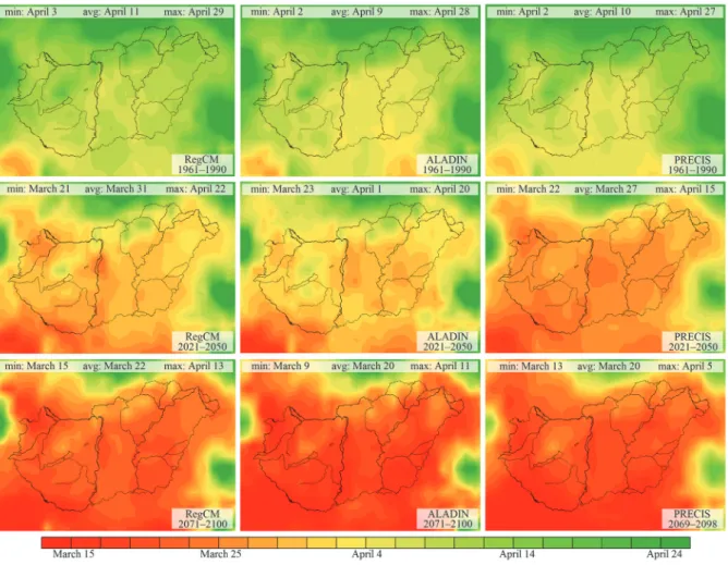
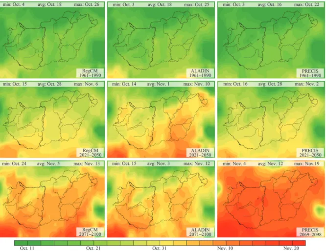
The average length (G_L;5mid) of growing seasons G_L^g_;5mid taken over all grid points g and for the reference period (R: 1961–1990) is 192 days (April 10 – October 18). Longer growing seasons (meaning earlier G_B^g_;5mid and later G_E^g_;5mid) occur typically in plain regions, while shorter growing seasons occur in hilly terrains. Such regional differences are projected for the 21st century (see Figs. 1 and 2). According to all three RCMs, the average growing season length (G_L;5mid) is 214 days (March 30 – October 29) in the time period 2021–2050.

RegCM and ALADIN simulation data show 229-day-long growing season (March 21 – November 4) up to the end of the 21st century. The PRECIS model simulation predicts that a 238-day-long growing season (March 20 – November 12) is also possible.

The calculation with the ‘int’ method shows similar spatial and temporal distributions. The length of the growing season has an average of 182–190 days (April 12 – October 15) in the reference period. RegCM and ALADIN simulations show a 201-day average growing season length (April 4 – October 21), while the PRECIS model estimates it to be 214 days long (March 31 – October 30) in the time period 2021–2050. For the end of the 21st century, RegCM and ALADIN outputs show an average of 210-day-long growing season (March 27 – October 22), and PRECIS simulation results with an up to 226-day- long growing season (March 25 – November 5).

These results suggest that because of the changing thermal conditions, the growing season is expected to be significantly longer in the middle and end of the 21st century, compared to what is calculated for (and observed at) the end of the 20th century. The beginning (the end) of the growing season tends to occur usually earlier (later) in the future, compared to what was experienced in the past.

Fig. 1. The beginning of the growing season (G_B^g_;5mid) in Hungary calculated with the

‘5mid’ method. Rows represent different time slices, i.e., 1961−1990 (upper row), 2021−2050 (middle row), and 2071−2100^* (lower row). Columns correspond to RegCM (left), ALADIN (middle), and PRECIS (right) simulations.

* 2069−2098 for the PRECIS model

Fig. 2. The end of the growing season (G_E^g_;5mid) in Hungary calculated with the ‘5mid’

method. Rows represent different time slices, i.e., 1961−1990 (upper row), 2021−2050 (middle row), and 2071−2100^* (lower row). Columns correspond to RegCM (left), ALADIN (middle), and PRECIS (right) simulations.

3.2. Adjusted Winkler index and adjusted Huglin’s heliothermal index (^AWIGSg and ^AHIGSg )

The average length of the growing season calculated with the ‘5mid’ method is usually longer than the one calculated with the ‘int’ method, therefore, the heat sum indicator values (AWI_GS^g and AHI_GS^g ) are evidently higher, with an average of 0–150 °C.

According to the RCMs, values of AWI_GS^g calculated for the reference period with the ‘5mid’ and ‘int’ methods are in the range of 833–1540 °C and 813–1501 °C, respectively. Higher values are usually in the plain regions, and lower values can be found in hilly terrains. Values of AWI_GS^g estimated for the middle of the 21st century can be as high as 1700–2000 °C in the southern part of the Great Hungarian Plain. The

* 2069−2098 for the PRECIS model

highest AWI_GS^g values at the end of the 21st century (‘5mid’: 1806–2657 °C; ‘int’:

1782–2607 °C) are projected by the PRECIS outputs, while the lowest values (‘5mid’:

1369–2248 °C; ‘int’: 1338–2161 °C) are predicted by the RegCM simulation.

Values of AHI_GS^g calculated for the reference period are 1363–2204 °C, and 1305–2161 °C calculated with the ‘5mid’ and ‘int’ (see Fig. 3) methods, respectively. Similarly to AWI_GS^g , higher values appear in the southern part of the Great Hungarian Plain. At the end of the 21st century, AHI_GS^g values are projected to exceed even 3000 °C in this region. RegCM simulation shows the smallest increase (600–800 °C increase) and PRECIS outputs show the largest increase (1000–1300 °C increase) by the end of the 21st century.

Values of AWI_GS^g (k) and AHI_GS^g (k) calculated with both methods (‘5mid’ and

‘int’) project significant (p < 0.05) increases from all examined time periods to later time period(s).

Fig. 3. Values of adjusted Huglin’s heliothermal index (AHI_GS^g , °C) in Hungary calculated with the ‘int’ method. Rows represent different time slices, i.e., 1961−1990 (upper row), 2021−2050 (middle row), and 2071−2100^* (lower row). Columns correspond to RegCM (left), ALADIN (middle), and PRECIS (right) simulations.

* 2069−2098 for the PRECIS model

3.3. Adjusted hydrothermal coefficient (AHTC_GS^g )

Values of AHTC_GS^g are in the range of 0.82–1.69 in Hungary in the reference period (see Fig. 4). High temperature with low precipitation (AHTC_GS^g values below 1.0) is usual in the plain regions, while AHTC_GS^g values above 1.0 appear in the hilly terrains. The RCM simulations predict decreasing AHTC_GS^g values (AHTC_GS^g : 0.54−1.44) during the 21st century. This prediction corresponds to a decrease of the dominance of temperature over precipitation, however, AHTC_GS^g values are not expected to fall into the critical interval (i.e., below 0.5).

) (k

AHTC_GS^g values predicted by PRECIS outputs for the end of the 21st century differ significantly (p < 0.05) from the estimated values of the reference period (see Fig. 5).

Fig. 4. Values of the adjusted hydrothermal coefficient (AHTC_GS^g ) in Hungary calculated with the ‘int’ method. Rows represent different time slices, i.e., 1961−1990 (upper row), 2021−2050 (middle row), and 2071−2100^* (lower row). Columns correspond to RegCM (left), ALADIN (middle), and PRECIS (right) simulations.

* 2069−2098 for the PRECIS model

Fig. 5. Comparison of the adjusted hydrothermal coefficient (AHTC_GS^g ) for Hungary calculated with the ‘int’ method. Rows represent different time slices, i.e., 1961−1990 (upper row), 2021−2050 (middle row), and 2071−2100^* (lower row). Columns correspond to RegCM (left), ALADIN (middle), and PRECIS (right) simulations. The different letters (or colors) show significantly different values with Bonferroni’s correction at the p<0.05 level.

3.4. Sum of precipitation (P_GS^g )

According to all three RCMs, values are in the range of 270−445 mm in Hungary in the time period 1961−1990. This amount is sufficient for the vital activities of grapevine (Kozma, 2002). P_GS^g (k) values do not show significant (p > 0.05) change for the 21st century. Results calculated from the RegCM outputs with the ‘5mid’

method show significant (p < 0.05) increase of P_GS^g (k) in the Transdanubian region and in northeastern Hungary during the 21st century.

* 2069−2098 for the PRECIS model

3.5. The length of the annual longest rainy and dry unbroken periods of precipitation (^LRPAg5_GS and ^LDPBg1_GS)

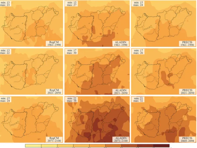
The distribution of precipitation during the year is also important for grapevine production. The projected changes of ^LRPAg5_GS(k) values are not significant (p > 0.05) in the investigated time period. The average values of ^LRPAg5_GS are 3–4 days. Statistically significant (p < 0.05) increase in the ^LDPBg1_GS(k) values is projected by ALADIN (using both the ‘5mid’ and ‘int’ methods) and PRECIS (using the ‘5mid’ method). ^LDPBg1_GS(k) values are estimated to increase from means of 12–29 days during the reference period to averages of 15–39 days by the end of the 21st century (see Fig. 6). Higher values are expected primarily in the region of the Great Hungarian Plain.

Fig. 6. Average length of the annual longest unbroken (dry) period of precipitation with below 1 mm per day during growing season (LDP_B^g_{1_GS}, day) in Hungary calculated with the ‘int’ method. Rows represent different time slices, i.e., 1961−1990 (upper row), 2021−2050 (middle row), and 2071−2100^* (lower row). Columns correspond to RegCM (left), ALADIN (middle), and PRECIS (right) simulations.

* 2069−2098 for the PRECIS model

3.6. The number of years with extreme high temperature (YN_A^g_{35_GS})

Extreme temperature indices as risk factors in grapevine production are also examined. According to RCM simulations, at least one day occurs every second or third year that has a maximum temperature above 35 °C in the reference period.

Such extreme events are most frequent in the southeastern and northwestern parts of Hungary. Day(s) with a maximum temperature above 35 °C are projected to occur in almost every year at the end of the 21st century.

3.7. The number of days with extreme low temperature (^DNBg1m_GSf ,^DNBg17m_D and ^DNBg21m_D)

The different RCM simulations and growing season calculation methods provide quite diverse results. The maximum value of DN_B^g_{1m_GSf} are 20 and 99 when using the ‘int’ method in case of the ALADIN and RegCM simulations, respectively.

Spatial distributions of DN_B^g_{1m_GSf}derived with different growing season calculation methods are also diverse. Using the ‘int’ method, we get lower values of DN_B^g_{1m_GSf}in plain regions are lower than in hilly terrains. Contrary to this, based on the ‘5mid’ method, values of DN_B^g_{1m_GSf} are usually higher in the plain regions.

On one hand, the PRECIS simulation predicts no day at all with a daily minimum temperature below −17 °C (−21 °C). On the other hand, DN_B^g_{17m_D} values are estimated in the range of 6−113 days (RegCM simulation) and 6−100 days (ALADIN simulation) for the reference period by the other two RCM simulations. The highest values appear in the Northern Hungarian Mountains.

According to both the RegCM and ALADIN simulations, the number of days with a daily minimum temperature below −17 °C may become zero during the 21st century. The likely range for DN_B^g_{17m_D}values by the end of the 21st century is 0−8 days.

g D m

DNB_{21 _} values are in the range of 0−20 days and 0−13 days (according to RegCM and ALADIN simulations, respectively) in the time period 1961−1990.

During the 21st century, these extreme temperature events are likely to disappear almost completely.

4. Discussion and conclusions

The aim of the presented study is to refine the growing season calculation methods based on fixed calendar days and find the most accurate ones (‘5mid’ and ‘int’) using the root-mean-square error compared to the reference growing season values based on averaging the daily mean temperature for several decades. The selected methods are able to handle the extreme temperature events. First we use

the ‘5mid’ and ‘int’ methods for the calculation of the beginning, the end, and the length of the growing season. We apply these methods to prepare some climatic indicators which are usually used in viticulture studies. In the calculations, a fixed biological base temperature (10 °C) is used for the grapevine (Amerine and Winkler, 1944; Winkler et al., 1974; Kozma, 2002). Our further aim is to sensitize the growing season calculation methods for different grapevine cultivars by modeling their special temperature demands (Hlaszny, 2012; Fraga et al., 2016).

Our results suggest that the growing season is to become significantly longer during the 21st century, which should be taken into account when calculating the growing season, and thus, should be adjusted to the thermal conditions. The increasing length of the growing season appears in a form of an earlier beginning and a later end.

Hungary is considered as a one of the countries close to the northern border of quality wine production (Schultz and Jones, 2010). Therefore, grapevine cultivar assortment is limited by climatic conditions. According to Van Leeuwen et al. (2008), grapevine cultivars have different heat requirements for their phenological stages, including the ripening time. The sum of heat claim has a large range across the varieties, from 1204 °C to 1940 °C for Chasselas and Mourvèdre, respectively. However, the necessary sum of heat for a given variety is not consistent for cool and warm climates.

The increase of heat sum indicator values (e.g., Huglin index) for the 21st century, is projected by regional climate models based on A1B scenario (Nakicenovic and Swart, 2000) in several studies for European wine regions (e.g., Malheiro et al., 2010; Neumann and Matzarakis, 2011). Based on the projection for the future, complex analyses of climatic indicators are necessary (Fraga et al., 2014).

Also, according to our results, values of heat sum indicators are expected to increase. Therefore, wide settlement and economical production of late-ripening and red grapevine cultivars with higher heat demand can become more likely in Hungary. Moreover, the length of periods with low precipitation and the occurrence frequency of days with extreme high temperature are expected to increase significantly, which are potential risk factors in grapevine production (Kozma, 2002). Nevertheless, a highly probable propitious effect is the projected significant decrease of winter frost damage events.

Acknowledgments: Simulation of the PRECIS regional climate model was supported by grant OTKA K-78125. The authors are grateful for Ildikó Pieczka (Eötvös Lorand University, Dpt. of Meteorology) for providing bias-corrected model outputs. The RegCM and ALADIN simulations were developed within the ENSEMBLES project (505539) which was funded by the EU FP6 integrated program. The E-OBS database was provided by the ENSEMBLES and ECA&D projects. This work has been supported by OTKA grants K109109 and K109361, and also by the Agrárklíma2 project (VKSZ_12-1- 2013-0034). The research was supported by the European Union and the European Social Fund (TÁMOP-4.2.1/B-09/1/KMR-2010-0003, FuturICT.hu grant no.: TÁMOP-4.2.2.C-11/1/KONV-2012- 0013), and by the Széchenyi 2020 programme, the European Regional Development Fund and the Hungarian Government (GINOP-2.3.2-15-2016-00028). We would also like to thank Peter Raffai for his valuable help with the English revision.

References

Ambrózy P., Bartholy J., Bozó L., Hunkár M.K., Bihari Z., Mika J., Németh P.R., Paál A., Szalai S., Kövér Zs., Tóth Z., Wantuch F., and Zoboki J., 2002: Magyarország éghajlati atlasza. Hungarian Meteorological Service, Budapest. (in Hungarian)

Amerine, M. A. and Winkler, A. J., 1944: Composition and quality of musts and wines of Californian grapes. Hilgardia 15, 493–675. https://doi.org/10.3733/hilg.v15n06p493

Bois, B., Blais, A., Moriondo, M., and Jones, G.V., 2012: High resolution climate spatial analysis of European winegrowing regions. IXe Intermational Terroirs Congress 2012, 17–20.

Csepregi P., 1997: Szőlőtermesztési ismeretek. Mezőgazda Kiadó, Budapest. (in Hungarian)

Davitaja, F., F. (Давитая, Ф., Ф.), 1959: Климатические показатели сьрьевой базы виноградо- винодельческой промышленности. Труды ВНИИВИВ „Магарач”, 6(1), 12–32. (in Russian) Déqué, M., Marquet, P., and Jones, R.G., 1998: Simulation of climate change over Europe using a global

variable resolution general circulation model. Clim. Dynam. 14, 173–189.

https://doi.org/10.1007/s003820050216

Dunkel, Z. and Kozma, F., 1981: A szőlő téli kritikus hőmérsékleti értékeinek területi eloszlása és gyakorisága Magyarországon. Légkör 26(2), 13–15. (in Hungarian)

Formayer, H., and Haas, P., 2010: Correction of RegCM3 model output data using a rank matching approach applied on various meteorological parameters. Deliverable D3.2 RCM output localization methods (BOKU-contribution of the FP 6 CECILIA project).

Fraga, H., Malheiro, A.C., Moutinho-Pereira, J., Jones, G.V., Alves, F., Pinto, J.G., and Santos, J.A., 2014: Very high resolution bioclimatic zoning of Portuguese wine regions: present and future scenarios. Reg. Environ. Change 14, 295–306. https://doi.org/10.1007/s10113-013-0490-y Fraga, H., Santos, J.A., Moutinho-Pereira, J., Carlos, C., Silvestre, J., Eiras-Dias, J., Mota, T., and

Malheiro, A.C., 2016: Statistical modelling of grapevine phenology in Portuguese wine regions:

observed trends and climate change projections. J. Agric. Sci. 154, 795–811.

https://doi.org/10.1017/S0021859615000933

Giorgi, F., Marinucci, M.R., Bates, G.T., and DeCanio, G., 1993: Development of a second generation regional climate model (RegCM2). Part II: Convective processes and assimilation of lateral boundary conditions. Mon. Weather Rev. 121, 2814–2832.

https://doi.org/10.1175/1520-0493(1993)121<2814:DOASGR>2.0.CO;2

Haylock, M.R., Hofstra, N., Klein Tank, A.M.G., Klok, E.J., Jones, P.D., and New, M., 2008: A European daily highresolution gridded data set of surface temperature and precipitation for 1950-2006.

Journal of Geophysical Research, Vol. 113, 1–12. https://doi.org/10.1029/2008JD010201 Hlaszny E., 2012: A szőlő (Vitis Vinifera L.) korai fenológiai válaszadásának modellezése a kunsági

borvidéken növényfelvételezések, időjárási megfigyelések és regionális klímamodell alapján.

Ph.D. thesis, Corvinus University of Budapest, Budapest. (in Hungarian)

Huglin, P., 1978: Nouveau mode d’évaluation des possibilités héliothermiques d’un milieo viticole.

Symposium International sur l’ecologie de la Vigne. Ministére de l’Agriculture et de l’Industrie Alimentaire, Contanca, 89–98. (in French)

IPCC, 2013: Climate Change 2013: The Physical Science Basis. Contribution of Working Group I to the Fifth Assessment Report of the Intergovernmental Panel on Climate Change (Eds. Stocker T.F., Qin D., Plattner G.-K., Tignor M., Allen S.K., Boschung J., Nauels A., Xia Y., Bex V., Midgley P.M.,).

Cambridge University Press, Cambridge, United Kingdom and New York, NY, USA.

Jones, G.V., Moriondo, M., Bois, B., Hall, A., and Duff, A., 2009: Analysis of the spatial climate structure in viticulture regions worldwide. Le Bulletin de l’OIV82(944,945,946), 507–518.

Kozma, P., 2002: A szőlő és termesztése I. Akadémiai Kiadó, Budapest. (in Hungarian)

van der Linden, P. and Mitchell, J.F.B., (Eds.), 2009: ENSEMBLES: Climate Change and Its Impacts:

Summary of research and results from the ENSEMBLES project. UK Met Office Hadley Centre, Exeter, UK.

Malheiro, A.C., Santos, J.A., Fraga, H., and Pinto, J.G., 2010: Climate change scenarios applied to viticultural zoning in Europe. Climate Res. 43, 163−177. https://doi.org/10.3354/cr00918

Mesterházy, I., Mészáros, R., and Pongrácz, R., 2014: The Effects of Climate Change on Grape production in Hungary. Időjárás 118, 193−206.

Moriondo, M., Jones, G.V., Bois, B., and Dibari, C., 2013: Projected shifts of wine regions in response to climate change. Climate Change 119, 825−839. https://doi.org/10.1007/s10584-013-0739-y Nakicenovic, N. and Swart, R.J., 2000: Emissions Scenarios 2000 – Special Report of the

Intergovernmental Panel on Climate Change. Cambridge University Press, Cambridge.

Neumann, P.A. and Matzarakis, A., 2011: Viticulture in southwest Germany under climate change conditions. Climate Res. 47, 161–169. https://doi.org/10.3354/cr01000

Oláh, L., 1979: Szőlészek zsebkönyve. Mezőgazdasági Kiadó, Budapest. (in Hungarian)

Pieczka, I., Pongrácz, R., Bartholy, J., Kis, A., and Miklós, E., 2011: A szélsőségek várható alakulása a Kárpát-medence térségében az ENSEMBLES projekt eredményei alapján. In (Ed.: Lakatos M.) 36. Meteorológiai Tudományos Napok - Változó éghajlat és következményei a Kárpát- medencében. Országos Meteorológiai Szolgálat, Budapest. 77–87. (in Hungarian)

Pieczka, I., 2012: A Kárpát-medence térségére vonatkozó éghajlati szcenáriók elemzése a PRECIS finom felbontású regionális klímamodell felhasználásával. Ph.D. thesis. Eötvös Loránd University, Department of Meteorology, Budapest. (in Hungarian)

Pongrácz, R., Bartholy, J., and Miklós, E., 2011: Analysis of projected climate change for Hungary using ENSEMBLES simulations. Appl. Ecol. Environ. Res. 9, 387–398.

https://doi.org/10.15666/aeer/0904_387398

Ramos, MC., Jones, G.V., and Martinez-Casasnovas, J.A., 2008: Structure and trends in climate parameters affecting winegrape production in northeast Spain. Climate Res. 38, 1–15.

https://doi.org/10.3354/cr00759

Riou, C., 1994: The Effect of Climate on Grape Ripening: Application to the Zoning of Sugar Content in the European Community. European Commission, Brussels, Luxembourg.

Santos, J.A., Malheiro, A.C., Pinto, J.G, and Jones, G.V., 2012: Macroclimate and viticultural zoning in Europe: observed trends and atmospheric forcing. Climate Res. 51, 89–103.

https://doi.org/10.3354/cr01056

Schultz, H.R. and Jones, G.V., 2010: Climate Induces Historic and Future Changes in Viticulture. J.

Wine Res. 21, 137−145. https://doi.org/10.1080/09571264.2010.530098

Seljaninov, G.T., 1928: О сельскохозяйственной оценке климата. Cельскохозяйственной метеорологии, 20, 165–177. (in Russian)

Szenteleki, K., Ladányi, M., Gaál, M., Zanathy, G., and Bisztray, Gy.D., 2012: Climatic risk factors of Central Hungarian grape growing regions. Appl. Ecol. Environ. Res. 10, 87–105.

https://doi.org/10.15666/aeer/1001_087105

Van Leeuwen, C., Garnier, C., Agut, C., Baculat, B., Barbeau, G., Besnard, E., Bois, B., Boursiquot J.- M., Chuine, I., Dessup, T., Dufourcq, T., Garcia-Cortazar, I., Marguerit, E., Monamy, C., Koundouras, S., Payan, J.-C., Parker, A., Renouf, V., Rodriguez-Lovelle, B., Roby, J.-P., Tonietto, J., and Trambouze, W., 2008: Heat requirements for grapevine varieties is essential information to adapt plant material in a changing climate. 7^th International Terroir Congress, Agroscope Changins-Wädenswil, Switzerland, 222–227.

Wilson, S., Hassell, D., Hein, D., Jones, R., and Taylor, R., 2007: Installing and using the Hadley Centre regional climate modelling system, PRECIS. Version 1.5.1. UK Met Office Hadley Centre, Exeter.

Winkler, A.J., Cook, J.A., Kliewer, W.M., and Lider, L.A., 1974: General Viticulture. University of California Press, California.