ANNALESMATHEMATICAEETINFORMATICAE33.(2006) Barrera-Figueroa, V., Sosa-Pedroza, J., López-Bonilla, J., Multi-
ple root finder algorithm for Legendre and Chebyshev polynomials via Newton’s method . . . 3 Bremner, A., On Heron triangles . . . 15 Čerin, Z., Gianella, G. M., Cyclic quadrangles from squares . . . 23 Fehér, Z., László, B., Mačaj, M., Šalát, T., Remarks on arithmetical
functions ap(n),γ(n),τ(n) . . . 35 Filip, F., Liptai, K., Tóth, J. T., On prime divisors of remarkable se-
quences . . . 45 Geda, G., Vágner, A., Solving ordinary differential equation systems by
approximation in a graphical way . . . 57 Grytczuk, A., Ljunggren’s Diophantine problem connected with virus struc-
ture . . . 69 Koumandos, S., Positive trigonometric sums and applications . . . 77 Mihály, T., Some properties of solutions of systems of neutral differential
equations . . . 93 Smith, S. J., Lebesgue constants in polynomial interpolation . . . 109 Sztrik, J., Kim, C. S., Performance modeling tools with applications . . . 125 Tómács, T., Líbor, Zs., A Hájek–Rényi type inequality and its applica-
tions . . . 141 Zsakó, L., Variations for spanning trees . . . 151
Methodological papers
Németh, B., Hoffmann, M., Gender differences in spatial visualization among engineering students . . . 169 Olajos, P., Orosz, E., Making slides for lecture by LATEX . . . 175 Szász, R., Mathematics teachers and differentiation - results of a survey
concerning Hungarian secondary schools . . . 189
HUNGARIA, EGER
ESZ
TERHÁZ YK ÁROLYCO LLEGE
EGE R 1774
S
ANNALES
MATHEMATICAE ET INFORMATICAE
TOMUS 33. (2006)
COMMISSIO REDACTORIUM
S´andor B´acs´o (Debrecen), Sonja Gorjanc (Zagreb), Tibor Gyim´othy (Szeged), Mikl´os Hoffmann (Eger), J´ozsef Holov´acs (Eger), L´aszl´o Kozma (Budapest), K´alm´an Liptai (Eger), Florian Luca (Mexico), Giuseppe Mastroianni (Potenza), Ferenc M´aty´as (Eger), ´Akos Pint´er (Debrecen), Mikl´os Ront´o (Miskolc, Eger),
J´anos Sztrik (Debrecen, Eger), Garry Walsh (Ottawa)
MATHEMATICAE ET INFORMATICAE
VOLUME 33. (2006)
EDITORIAL BOARD
Sándor Bácsó (Debrecen), Sonja Gorjanc (Zagreb), Tibor Gyimóthy (Szeged), Miklós Hoffmann (Eger), József Holovács (Eger), László Kozma (Budapest), Kálmán Liptai (Eger), Florian Luca (Mexico), Giuseppe Mastroianni (Potenza), Ferenc Mátyás (Eger), Ákos Pintér (Debrecen), Miklós Rontó (Miskolc, Eger),
János Sztrik (Debrecen, Eger), Garry Walsh (Ottawa)
INSTITUTE OF MATHEMATICS AND COMPUTER SCIENCE ESZTERHÁZY KÁROLY COLLEGE
HUNGARY, EGER
A kiadásért felelős:
az Eszterházy Károly Főiskola rektora Megjelent az EKF Líceum Kiadó gondozásában
Kiadóvezető: Kis-Tóth Lajos Felelős szerkesztő: Zimányi Árpád Műszaki szerkesztő: Tómács Tibor Megjelent: 2007. január Példányszám: 50 Készítette: Diamond Digitális Nyomda, Eger
Ügyvezető: Hangácsi József
http://www.ektf.hu/tanszek/matematika/ami
Multiple root finder algorithm for Legendre and Chebyshev polynomials via Newton’s
method
Victor Barrera-Figueroa
a, Jorge Sosa-Pedroza
b, José López-Bonilla
cabcInstituto Politécnico Nacional, Escuela Superior de Ingeniería Mecánica y Eléctrica, Sección de Estudios de Postgrado e Investigación
ae-mail: vbarreraf@ipn.mx;be-mail:jsosa@ipn.mx;ce-mail:jlopezb@ipn.mx Submitted 23 June 2006; Accepted 31 October 2006
Abstract
We exhibit a numerical technique based on Newton’s method for finding all the roots of Legendre and Chebyshev polynomials, which execute less itera- tions than the standard Newton’s method and whose results can be compared with those for Chebyshev polynomials roots, for which exists a well known analytical formula. Our algorithm guarantees at least nine decimal correct ciphers in the worst case, however, when comparing with Chebyshev roots given by its formula, even eighteen decimal correct ciphers are achieved in several roots, in the best case. As a comparison guide the results are collated with those gotten by MATLAB.
Keywords: Newton’s method, Legendre polynomials, Chebyshev polynomi- als, multiple root finder algorithm.
1. Introduction
Legendre polynomials (see [1, 2, 3, 4]) as well as Chebyshev (see [1, 2, 3, 4, 5]) ones has found countless applications in all branches of engineering and sci- ence, among which the most representatives include calculation of quadratures, electromagnetics and antenna applications, solutions for potential theory and for Schrödinger’s equation, aerodynamics and mechanics applications, etc. This is due mainly because the use of their roots allows us to solve a specific problem with the best efficiency.
These polynomials are very similar to each other, not only in the form of their respective differential equation, but also in the numerical values of their roots.
3
However, sometimes it is better the use of Legendre polynomials instead of Cheby- shev ones because by using their roots, one can reach the most optimized solution.
For instance, when calculating a quadrature, Gauss established that the best way for obtaining the minimum error in a numerical integration is by dividing the inte- gration domain in agreement with the way Legendre roots are distributed on their own domain.
So, because of the wide use of Legendre and Chebyshev roots, this paper presents a multiple root finder algorithm, which is expected to be a useful tool, not only in engineering work but also in numerical and mathematical analysis. This algorithm is based in the classical Newton’s method (see [2]), however, we have made some modifications in order to find all the roots of an specific polynomial by using the improved Newton’s method (see [2]).
2. Newton’s method
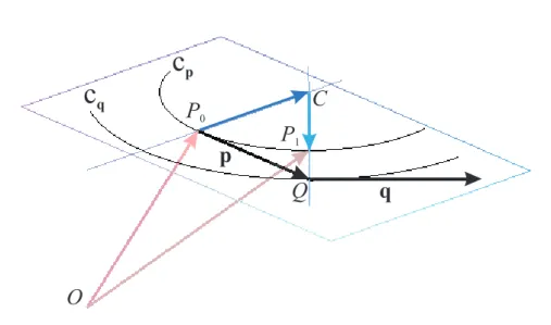
Newton’s process is a numerical tool used to find the zero xe of a real-valued functionf(x), continuously differentiable and whose derivative does not vanish at x=xe. The method consists in proposing an initial rootx0 which must be in the neighborhood ofxe, as shown in Figure 1. Once made this, we draw a tangent line tof(x)atx=x0, and determine its intersection with thexaxis. The equation for the line is:
y=f(x0) +f′(x0)(x−x0), (2.1) which means that locally, in the small neighborhood of x0,f(x)can be considered as a linear equation, even iff(x)is not linear. We should notice that this equation corresponds to the truncate Taylor series with center at x=x0 by neglecting the remainder term. The intersection, named x1, is then:
x1−x0=−f(x0)
f′(x0), (2.2)
Now,x1is closer to the real zeroxe, and it will be used to draw the next tangent line tof(x)atx=x1 which produces the intersectionx2. So, in thenthiteration, the intersection of the tangent line with thexaxis will be [2]:
xn=xn−1− f(xn−1)
f′(xn−1), n= 1,2,3, . . . (2.3) After a number of iterations xn will be close enough to xe. In this way, once we have established the allowed error ǫfor the zero, we can set the condition for stopping the method, which is reached when:
|xn−xn−1|6ǫ. (2.4)
Newton’s technique will usually converge provided the initial guess is close enough to true root. Furthermore, for a zero of multiplicity 1, the convergence
Figure 1: Tangent lines tof(x)atx=x1.
is at least quadratic in a neighborhood of xe, which intuitively means that the number of correct digits roughly at least doubles in every step.
Newton’s method acquire a bigger convergence if in Taylor series we consider the quadratic term:
y=f(x0) +f′(x0)(x−x0) +1
2f′′(x0)(x−x0)2, (2.5) that is, in the small neighborhood of x0, f(x) can be considered as a quadratic equation, even iff(x)is not quadratic. The intersection x1 between (2.5) and the xaxis can be calculated from:
x1−x0=− f(x0)
f′(x0) +12f′′(x0)(x1−x0), (2.6) by substituting (2.2) into (2.6) we get:
x1−x0=− 2f(x0)f′(x0)
2 [f′(x0)]2−f(x0)f′′(x0). (2.7) So, in thenthiteration, we have the next recursive formula (see [2]):
xn=xn−1− 2f(xn−1)f′(xn−1)
2 [f′(xn−1)]2−f(xn−1)f′′(xn−1), n= 1,2,3, . . . (2.8) This is the improved Newton’s method which converges faster than the original one. As well as we have to know the first derivative of f(x)in both methods, in the improved one, we must know the second derivative off(x)in each point. This could be a problem if f(x)is not an analytical formula but a set of data points, in which both derivatives could be calculated from standard numerical techniques.
3. Multiple root finder algorithm based on Newton’s process
The application of Newton’s method to a polynomial in the quest for all its roots could be easily implemented if we express it according to the fundamental theorem of Algebra:
f(x) =k(x−x1)(x−x2). . .(x−xN), (3.1) where N is the polynomial order, k is a proportionality constant and {x1, x2, . . . , xN} are all the polynomial roots, which are not necessarily put in order. In the following, the subindexj in the rootxj represents the number of root and it should not be confused with the number of iterations used in the previous sections which will be omitted from here. By applying Newton’s algorithm to the polynomial (3.1) for searching the first rootx1, we have the next recursive relation:
x1=x1− f(x)
f′(x). (3.2)
Oncex1 is found, we built the polynomial g(x)of orderN −1 which has not x1 as one of its roots:
g(x) = f(x) x−x1
=k(x−x2)(x−x3). . .(x−xN), (3.3) and by applying Newton’s technique tog(x)we determine the next rootx2and so on. So, in thekthstep, we built the following polynomial:
g(x) = f(x) Qk−1
i=1(x−xi), (3.4)
and, according to Newton’s method, thekth root is:
xk =xk− g(xk)
g′(xk), (3.5)
which implies the calculation for the derivative ofg(x)which could not be so evident because of the need to find the derivative of the product term. Such derivative is:
d dx
kY−1 i=1
(x−xi) = 1
x−x1
+ 1
x−x2
+· · ·+ 1 x−xk−1
kY−1 i=1
(x−xi) =
=
kY−1 i=1
(x−xi)
k−1
X
i=1
1 x−xi
, (3.6)
therefore the derivative forg(x)is:
g′(x) = 1 Qk−1
i=1(x−xi)
"
f′(x)−f(x)
k−1
X
i=1
1 x−xi
#
. (3.7)
By substituting (3.7) and (3.4) into (3.5) we reach the recursive relation for getting all the roots for the polynomialf(x):
xk =xk− f(xk) f′(xk)−f(xk)Pk−1
i=1 1 x−xi
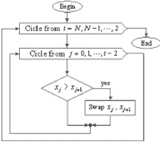
, k= 1,2, . . . , N. (3.8) On the basis of (3.8) we express the multiple root finder algorithm with the following diagram:
Figure 2: Multiple root finder algorithm.
In order to sort all the roots given by the multiple root finder process, we can introduce the well known bubble sort method which by successively interchanging theN roots can provide us the list of expected results. The bubble sort method is drawn in the following diagram:
4. Multiple root finder algorithm based on improved Newton’s method
In order to improve the algorithm’s convergence, we can introduce Newton’s technique in the quest for all the polynomial roots. In first term we look at the
Figure 3: Bubble sort method for putting in order the polynomial’s roots.
rootx1 of the polynomial (3.1) with the recursive relation (2.8). Oncex1is found, we built the polynomial g(x), (3.3). By applying improved Newton’s method to g(x) we found the next root x2 and so on. So, in the kth step, we built the polynomial (3.4), from which thekthroot is:
xk=xk− 2g(xk)g′(xk)
2 [g′(xk)]2−g(xk)g′′(xk). (4.1) Iterative formula (4.1) implies the calculation for the second derivative ofg(x) which could a hard task, however, the result is not as difficult as one could expect:
g′′(x) =
f′′(x)−2f′(x)kP−1
i=1 1
x−xi +f(x)
"
kP−1 i=1
1 (x−xi)2 +
k−1 P
i=1 1 x−xi
2#
kQ−1 i=1
(x−xi)
. (4.2)
So by substituting (3.4),(3.7) and (4.2) into (4.1) we get:
xk=xk− 2f(xk)B(xk)
B2(xk) + [f′(xk)]2−f(xk)
f′′(xk) +f(xk)
kP−1 i=1
1 (xk−xi)2
, (4.3)
B(xk) =f′(xk)−f(xk)
k−1
X
i=1
1 xk−xi
, k= 1,2, . . . , N.
Notice the similarity between (4.1) and (4.3) where f(xk) is similar to g(xk), and g′(xk) is analogous to B(xk). Obviously both formulas are not completely analogous, but the existent similarity is notorious. On the basis of (4.3) we express the improved multiple root finder algorithm with the following diagram, Figure 4, again, the bubble sort method could be used in order to sort the obtained roots:
Figure 4: Improved multiple root finder algorithm.
5. Legendre and Chebyshev polynomials roots cal- culation
In this section we present the results reached by both algorithms applied to Legendre and Chebyshev polynomials; also, it is shown the number of performed iteration. Such results are compared with those gotten by MATLAB. In the case of Chebyshev’s roots, we provide the analytical results gotten by the formula [2]:
xk= cos
2k−1 2N π
, k= 1,2, . . . , N, (5.1) whereN is the polynomial degree. Legendre polynomialsPn(x)are the solution of the Legendre differential equation:
(1−x2)d2Pn(x)
dx2 −2xdPn(x)
dx +n(n+ 1)Pn(x) = 0, n= 0,1,2, . . . , (5.2)
while Chebyshev polynomialsTn(x)are the solution for its respective differential equation:
(1−x2)d2Tn(x)
dx2 −xdTn(x)
dx +n2Tn(x) = 0, n= 0,1,2, . . . . (5.3) Both Pn(x)and Tn(x)can be defined by mean of recursive relations, which is an important issue in the numerical point of view. For Legendre polynomials, the recursive relations are:
P0(x) = 1, P1(x) =x, Pn+2=2n+ 3
n+ 2 xPn+1−n+ 1
n+ 2Pn, n= 0,1,2, . . . , (5.4) while for Chebyshev polynomials the recursive relations are:
T0(x) = 1, T1(x) =x, Tn+2= 2xTn+1−Tn, n= 0,1,2, . . . , (5.5) Such polynomials are plotted in Figure 5. It is notable how the roots are clustered in the ends of the domain [−1,1]in both polynomials.
Figure 5: Legendre and Chebyshev polynomials.
In Table 1 are shown the results forP19(x) roots reached by both algorithms, with a permissible error ofǫ= 1×10⁻¹² for each of them.
In Table 2 the roots for P19(x) obtained using MATLAB are presented for comparison. In Table 3 are shown the results for T19(x) roots reached by both algorithms, with a permissible error ofǫ= 1×10⁻¹² for each of them.
In Table 4 the roots forT19(x)obtained using (5.1) and MATLAB are presented for comparison.
6. Conclusions
Both algorithms have shown to be effective in finding all the roots for a specific polynomial. Such polynomial must have all its roots real and with simple mul- tiplicity. These conditions are satisfied by Legendre and Chebyshev polynomials.
Multiple root finder Number of Improved multiple root Number of
k algorithm,xk iterations finder algorithm,xk iterations
1 -0.992406843843584352 2 -0.992406843843584350 3 2 -0.960208152134830018 12 -0.960208152134830020 4 3 -0.903155903614817901 15 -0.903155903614817900 7 4 -0.822714656537142819 6 -0.822714656537142820 4 5 0.720966177335229386 6 -0.720966177335229390 4 6 -0.600545304661680990 6 -0.600545304661680990 5 7 -0.464570741375960938 7 -0.464570741375960940 5 8 -0.316564099963629830 8 -0.316564099963629830 6 9 -0.160358645640225367 9 -0.160358645640225390 6 10 0.000000000000000000 10 0.000000000000000000 6 11 0.160358645640225367 10 0.160358645640225390 7 12 0.316564099963629830 11 0.316564099963629830 7 13 0.464570741375960938 11 0.464570741375960940 7 14 0.600545304661680990 12 0.600545304661680990 8 15 0.720966177335229386 11 0.720966177335229390 8 16 0.822714656537142819 11 0.822714656537142820 8 17 0.903155903614817901 10 0.903155903614817900 7 18 0.960208152134830018 8 0.960208152134830020 7 19 0.992406843843584352 8 0.992406843843584460 5
Table 1: Roots forP19(x)with both algorithms.
However, for other type of polynomials, another process is being developed in order to get not only their real roots but also their complex ones, taking into account their own multiplicity.
The first algorithm is faster than the second one, because it performs fewer operations than the improved one, which must calculate the second derivative and several sums, among other operations. However, the second algorithm executes less iteration than the first one, and this fact could be useful in finding the roots for polynomials of big order. Both algorithms provide us several correct ciphers when comparing with the results gotten by MATLAB, however, both are faster than the routines used by MATLAB in doing the same action.
It is expected that these algorithms can be employed as a part for several programs which must involve quadratures or interpolations (among other numerical issues) while looking for engineering or science solutions, because of its speed and ease for programming. We the authors recommend an error of ǫ= 1×10⁻¹² for each root, which has shown to provide correct results for all the possible polynomial degrees. However, for an error of ǫ= 1×10⁻¹⁸ in some degrees, both algorithms perform a great number of iterations in which the loop becomes endless.
k MATLAB,xk
1 -0.992406843843584350 2 -0.960208152134830020 3 -0.903155903614817900 4 -0.822714656537142820 5 -0.720966177335229390 6 -0.600545304661680990 7 -0.464570741375960940 8 -0.316564099963629830 9 -0.160358645640225370 10 0.000000000000000000 11 0.160358645640225370 12 0.316564099963629830 13 0.464570741375960940 14 0.600545304661680990 15 0.720966177335229390 16 0.822714656537142820 17 0.903155903614817900 18 0.960208152134830020 19 0.992406843843584350 Table 2: Roots forP19(x)with MATLAB.
Multiple root finder Number of Improved multiple root Number of
k algorithm,xk iterations finder algorithm,xk iterations
1 -0.996584493006669847 2 -0.996584493006669850 3 2 -0.969400265939330374 12 -0.969400265939330370 5 3 -0.915773326655057396 15 -0.915773326655057400 7 4 -0.837166478262528546 4 -0.837166478262528550 4 5 -0.735723910673131587 5 -0.735723910673131590 4 6 -0.614212712689667817 6 -0.614212712689667820 4 7 -0.475947393037073563 7 -0.475947393037073560 5 8 -0.324699469204683511 8 -0.324699469204683510 5 9 -0.164594590280733893 9 -0.164594590280733890 6 10 0.000000000000000000 10 0.000000000000000000 6 11 0.164594590280733893 10 0.164594590280733890 7 12 0.324699469204683511 11 0.324699469204683460 7 13 0.475947393037073563 11 0.475947393037073560 7 14 0.614212712689667817 12 0.614212712689667820 8 15 0.735723910673131587 12 0.735723910673131590 8 16 0.837166478262528546 11 0.837166478262528550 8 17 0.915773326655057396 10 0.915773326655057400 7 18 0.969400265939330374 8 0.969400265939330370 7 19 0.996584493006669847 8 0.996584493006669850 5
Table 3: Roots forT19(x)with both algorithms.
Analytical formula:
k xk = cos 2k2N−1π
MATLAB,xk
1 -0.996584493006669847 -0.996584493006669850 2 0.969400265939330486 -0.969400265939330370 3 -0.915773326655057507 -0.915773326655057510 4 -0.837166478262528546 -0.837166478262528550 5 -0.735723910673131587 -0.735723910673131590 6 -0.614212712689667817 -0.614212712689667820 7 -0.475947393037073563 -0.475947393037073560 8 -0.324699469204683455 -0.324699469204683460 9 -0.164594590280733838 -0.164594590280734060 10 0.000000000000000061 0.000000000000000061 11 0.164594590280733977 0.164594590280733980 12 0.324699469204683566 0.324699469204683570 13 0.475947393037073618 0.475947393037073620 14 0.614212712689667817 0.614212712689667820 15 0.735723910673131698 0.735723910673131590 16 0.837166478262528657 0.837166478262528550 17 0.915773326655057396 0.915773326655057400 18 0.969400265939330374 0.969400265939330370 19 0.996584493006669847 0.996584493006669850 Table 4: Roots forT19(x)with analytical formula and MATLAB.
References
[1] M. Abramowitz and I. A. Stegun,Handbook of mathematical functions, Wiley and Sons, N. Y. (1972).
[2] C. Lanczos,Applied analysis, Dover N. Y. (1988).
[3] J. B. Seaborn,Hypergeometric functions and their applications, Springer-Verlag (1991).
[4] C. Lanczos, Linear differential operators, Dover N. Y. (1997).
[5] J. C. Mason and D. C. Handscomb, Chebyshev polynomials, Chapman&Hall - CRC Press (2002).
V. Barrera-Figueroa, J. Sosa-Pedroza, J. López-Bonilla UPALM. Edif. Z-4, 3er. piso, col. Lindavista, C.P. 07738, México D.F.
http://www.ektf.hu/tanszek/matematika/ami
On Heron triangles
Andrew Bremner
Department of Mathematics and Statistics, Arizona State University e-mail: bremner@asu.edu
Submitted 30 August 2006; Accepted 15 November 2006
Abstract
There has previously been given a one-parameter family of pairs of Heron triangles with equal perimeter and area. In this note, we find two two- parameter families of such triangle pairs, one of which contains the known one-parameter family as a special case. Second, for an arbitrary integern>2 we show how to find a set ofn Heron triangles in two parameters such that all triangles have equal perimeter and area.
MSC:11D72, 14G05.
1. Introduction
A.-V. Kramer and F. Luca [3] investigate several problems related to Heron tri- angles (triangles with integral sides and integral area; rationaltriangles are those with rational sides and rational area, which by scaling thus become Heron trian- gles). They give a one-parameter family of pairs of such triangles having equal perimeter and area (curiously, Aassila [1] in a paper that gives the appearance of plagiarism produces exactly the same parametric family). This note shows first in completely elementary manner how to construct a doubly infinite family of such tri- angle pairs. In fact we produce two such parametrizations, in three (homogeneous) parameters, containing the Kramer-Luca family as a special case.
Recently, van Luijk [4] answers a question posed by Kramer and Luca by show- ing that there exist arbitarily many Heron triangles having equal perimeter and area, and gives a method whereby a one-parameter family may be written down for nsuch triangles for a given integer n. We use the same ideas in showing how to produce a set ofnHeron triangles in two parameters with the property of equal perimeter and area.
15
2. Pairs of Heron triangles
Brahmagupta gave a parametrization for all Heron triangles, with sides propor- tional to
(v+w)(u2−vw), v(u2+w2), w(u2+v2),
where the semi-perimeter is equal tou2(v+w), and the area is equal to uvw(v+ w)(u2−vw). Thus to find a pair of Heron triangles with equal perimeter and area, we take the two triangles with independent parameters u, v, wandr, s, tand demand solutions of the system
u2(v+w) =mr2(s+t), uvw(v+w)(u2−vw) =m2rst(s+t)(r2−st), for a scaling factor m. The general solution will be difficult to obtain. However, we focus on the situationu=rand consider two cases.
First,m= 1. Thenw=s+t−v and equality of the area demands (s+t)u(s−v)(t−v)(st−u2+sv+tv−v2) = 0.
For non-trivial solutions, we thus havest−u2+sv+tv−v2= 0, and this quadric surface is birationally equivalent to the projective plane under the mapping
s:t:u:v=b(b+c) : (a2−bc+c2) :a(b+c) :c(b+c), (with inverse a:b:c=u:s:v). Accordingly,
r:s:t:u:v:w=a(b+c) :b(b+c) :a2−bc+c2:a(b+c) :c(b+c) :a2+b2−bc, leading to the triangle-pair
b(a2−bc+c2)(a2+b2+c2),
c(a4+ 3a2b2+b4−2b3c+a2c2+b2c2),
(b+c)(a2+b2−bc)(a2+c2), (2.1) and
c(a2+b2−bc)(a2+b2+c2),
b(a4+a2b2+ 3a2c2+b2c2−2bc3+c4),
(a2+b2)(b+c)(a2−bc+c2) (2.2) with the common semi-perimeter a2(b+c)(a2+b2+c2) and the common area abc(b+c)(a2+b2−bc)(a2−bc+c2)(a2+b2+c2). As an example, at(a, b, c) = (2,3,4), we obtain the triangles (174,197,35)and (29,195,182), both with perimeter 406 and area 2436.
Second, we assume m 6= 1 and restrict to v = ms, w = mt, when the perime- ters become equal. Equality of the area demands
−r2+st+mst+m2st= 0,
and considered as a quadric curve overQ(m)we have a birational correspondence with the projective line given by
r:s:t= (1 +m+m2)πρ: (1 +m+m2)ρ2:π2, π:ρ=r:s.
Thus
r:s:t:u:v:w=
(1 +m+m2)πρ: (1 +m+m2)ρ2:π2: (1 +m+m2)πρ:m(1 +m+m2)ρ2:mπ2= P(Q2+QR+R2) :R(Q2+QR+R2) :P2R:P(Q2+QR+R2) :Q(Q2+QR+R2) :P2Q,
on settingπ/ρ=P/R,m=Q/R(soP, Q, Rindependent parameters). This leads to the triangle pair
Q(Q+R)(P2+Q2+QR+R2),
Q4+ 2Q3R+P2R2+ 3Q2R2+ 2QR3+R4,
(P2+R2)(Q2+QR+R2) (2.3)
and
R(Q+R)(P2+Q2+QR+R2),
P2Q2+Q4+ 2Q3R+ 3Q2R2+ 2QR3+R4,
(P2+Q2)(Q2+QR+R2). (2.4)
If we put(P, Q, R) = (t(3 + 3t2+t4),1,1 +t2), then the resulting triangle pair is the one-parameter family of Kramer and Luca [3].
3. Sets of Heron triangles
Kramer and Luca [3] essentially ask whether one can find sets ofk Heron tri- angles with equal perimeter and area, for a given positive integerk. Relatedly, for a given triangle with rational sides a0, b0, c0 of perimeter 2s and area A, we can ask to find other triangles with the same perimeter and area. If such a triangle has sidesa, b, cthen
a+b+c= 2s, s(s−a)(s−b)(s−c) =A2. Equivalently,
C:s(s−a)(s−b)(a+b−s) =A2, (3.1) the equation of a cubic curve in the a, b-plane. CertainlyCcontains the points at infinity(0,1,0),(1,0,0),(−1,1,0), so is an elliptic curve. Fixing one of these points
as the zero of the group law, then the other two points become torsion points of order 3. Moreover, C contains the rational points at (a, b) = (a0, b0), (b0, a0), (b0, c0), (c0, b0), (c0, a0), (a0, c0), the sextet comprising the points ±(a0, b0) + 3- torsion in the group C(Q). In general, the point (a0, b0)will be of infinite order, allowing arbitrarily large sets of rational points (a, b) to be determined, each in turn defining a triangle with sides (a, b,2s−a−b), having the perimeter 2s and area A. The triangle may of course not be geometrically realisable ifa <0,b <0, or2s < a+b, or if the triangle inequality is violated; but since(a0, b0)corresponds to a genuine triangle, a density argument of points on the elliptic curve (dating back to Hurwitz: see Theorem 13 of [2]) guarantees the existence of arbitrarily many(a, b)corresponding to genuine triangles. (van Luijk [4] makes this argument explicit: if points Pi correspond to real triangles, then Pi=k
i=1niPi corresponds to a real triangle if and only if Pi=k
i=1ni is odd). Scaling will now produce arbitrarily large sets of Heron triangles with equal perimeter and area.
Remark 3.1. The isosceles triangle (a0, a0, c0) with b0 = a0 has corresponding curveC with (homogeneous) equation
2ab(a+b)−(2a0+c0)(a2+3ab+b2)d+(2a0+c0)2(a+b)d2−a0(2a20+3a0c0+2c20)d3= 0, and the points(a0, a0),(a0, c0), and(c0, a0)have the property that doubling them results in a torsion point at infinity: so the points are either of order 2 or of order 6. The point (a0, b0) may also be of finite order for a non-isosceles triangle, for example the triangle (a0, b0, c0) = (13,27,34), where (a0, b0) has order 12. If the rational rank of C is 0 (as is the case for example with the (non-Heron) triangles given by(a0, b0, c0) = (1,1,1) or(13,27,34)) then there are at most finitely many rational-sided triangles with same perimeter and area, arising from the torsion points on C. When (a0, b0) is a torsion point therefore, to determine arbitrarily many triangles with equal perimeter and area we requireC to have an additional rational non-torsion point (corresponding to a real triangle) in order to start the above construction. For instance, the Heron triangle (14,25,25) has (a0, b0) a torsion point, but the respective curveCexhibits the additional non-torsion point
39 2,1365
, leading to the triangle 392,1365 ,17310
, with same perimeter and area.
As illustration of the above construction of sets of points, take as example the Heron triangle (3,4,5), with semi-perimeter 6 and area 6. The construction of taking multiples of the point (3,4) onC provides the triangles
156 35,41
15,101 21
,
81831 16159,27689
8023 ,35380 10153
,
678541575
151345267,683550052
142637329,221167193 81180907
, . . .
with perimeter 6 and area 6. The numbers grow rapidly because the underlying elliptic curve here has rank 1, and the heights on an elliptic curve of multiples of a fixed point are rapidly increasing. When the underlying curve has higher rank, then by taking linear combinations of the generators there is expectation of a greater supply of rational points with relatively small height, and accordingly an
expectation of a more plentiful supply of triangles, as for example in the table of van Luijk [4], where 20 triangles are generated with same area and perimeter as the triangle(75,146,169); in this instance, the underlying elliptic curve has rank4 (independent points onC are(111,104),(125,91),(146,75), and(265,203)).
Of course, we can use as our initial triangle one given by a one- or two-parameter family, and construct arbitrarily many triangles in the corresponding number of parameters, all having the same perimeter and area. The formulae rapidly become lengthy, and we give as example a three (homogeneous) parameter family of only four such triangles, arising from the parametrizations at (2.3), (2.4). Denote the points onCcorresponding to the parametrizations (2.3), (2.4), bySandT respec- tively. Then the parametrizations corresponding to the pointsS,T,2S+T,S+ 2T are given by:
Q(Q+R)(2Q+R)(Q+ 2R)(P2+Q2+QR+R2)(P2Q+Q3+P2R+Q2R+QR2)(P2Q+P2R+
Q2R+QR2+R3)(P2Q+Q3+ 2Q2R+ 2QR2+R3)(Q3+P2R+ 2Q2R+ 2QR2+R3), (2Q+R)(Q+ 2R)(P2Q+Q3+P2R+Q2R+QR2)(P2Q+P2R+Q2R+QR2+R3)(P2Q+Q3+
2Q2R+ 2QR2+R3)(Q3+P2R+ 2Q2R+ 2QR2+R3)(Q4+ 2Q3R+P2R2+ 3Q2R2+ 2QR3+R4), (2Q+R)(Q+ 2R)(P2+R2)(Q2+QR+R2)(P2Q+Q3+P2R+Q2R+QR2)(P2Q+P2R+
Q2R+QR2+R3)(P2Q+Q3+ 2Q2R+ 2QR2+R3)(Q3+P2R+ 2Q2R+ 2QR2+R3),
R(Q+R)(2Q+R)(Q+ 2R)(P2+Q2+QR+R2)(P2Q+Q3+P2R+Q2R+QR2)(P2Q+P2R+
Q2R+QR2+R3)(P2Q+Q3+ 2Q2R+ 2QR2+R3)(Q3+P2R+ 2Q2R+ 2QR2+R3), (2Q+R)(Q+ 2R)(P2Q+Q3+P2R+Q2R+QR2)(P2Q+P2R+Q2R+QR2+R3)(P2Q+Q3+
2Q2R+ 2QR2+R3)(Q3+P2R+ 2Q2R+ 2QR2+R3)(P2Q2+Q4+ 2Q3R+ 3Q2R2+ 2QR3+R4), (P2+Q2)(2Q+R)(Q+ 2R)(Q2+QR+R2)(P2
Q+Q3+P2 R+Q2
R+QR2)(P2
Q+P2R+
Q2R+QR2+R3)(P2Q+Q3+ 2Q2R+ 2QR2+R3)(Q3+P2R+ 2Q2R+ 2QR2+R3),
(2Q+R)(P2Q+Q3+P2R+Q2R+QR2)(P2Q+Q3+ 2Q2R+ 2QR2+R3)(Q3+P2R+ 2Q2R+
2QR2+R3)(P4Q4+P2Q6+ 4P4Q3R+ 6P2Q5R+ 6P4Q2R2+ 13P2Q4R2+ 4P4QR3+ 16P2Q3R3+P4R4+ 13P2Q2R4+Q4R4+ 6P2QR5+ 2Q3R5+ 2P2R6+ 3Q2R6+ 2QR7+R8), (2Q+R)(P2Q+Q3+P2R+Q2R+QR2)(P2Q+P2R+Q2R+QR2+R3)(P2Q+Q3+ 2Q2R+
2QR2+R3)(P2Q6+Q8+ 6P2Q5R+ 6Q7R+ 13P2Q4R2+ 17Q6R2+ 16P2Q3R3+ 30Q5R3+ P4R4+ 13P2Q2R4+ 36Q4R4+ 6P2QR5+ 30Q3R5+ 2P2R6+ 17Q2R6+ 6QR7+R8), R(Q+R)(2Q+R)(Q+ 2R)(Q2+QR+R2)(P2+Q2+QR+R2)(P2Q+Q3+P2R+Q2R+QR2)
(P2Q+Q3+ 2Q2R+ 2QR2+R3)(P4
−P2Q2+Q4+ 2P2QR+ 2Q3R+ 2P2R2+ 3Q2R2+ 2QR3+R4),
(Q+ 2R)(P2Q+P2R+Q2R+QR2+R3)(P2Q+Q3+ 2Q2R+ 2QR2+R3)(Q3+P2R+ 2Q2R+
2QR2+R3)(P4Q4+ 2P2Q6+Q8+ 4P4Q3R+ 6P2Q5R+ 2Q7R+ 6P4Q2R2+ 13P2Q4R2+ 3Q6R2+ 4P4QR3+ 16P2Q3R3+ 2Q5R3+P4R4+ 13P2Q2R4+Q4R4+ 6P2QR5+P2R6),
(Q+ 2R)(P2Q+Q3+P2R+Q2R+QR2)(P2Q+P2R+Q2R+QR2+R3)(Q3+P2R+ 2Q2R+
2QR2+R3)(P4Q4+ 2P2Q6+Q8+ 6P2Q5R+ 6Q7R+ 13P2Q4R2+ 17Q6R2+ 16P2Q3R3+ 30Q5R3+ 13P2Q2R4+ 36Q4R4+ 6P2QR5+ 30Q3R5+P2R6+ 17Q2R6+ 6QR7+R8), Q(Q+R)(2Q+R)(Q+ 2R)(Q2+QR+R2)(P2+Q2+QR+R2)(P2Q+P2R+Q2R+QR2+R3)
(Q3+P2R+ 2Q2R+ 2QR2+R3)(P4+ 2P2Q2+Q4+ 2P2QR+ 2Q3R−P2R2+ 3Q2R2+ 2QR3+R4).
Remark 3.2. The family of elliptic curves at (3.1) is actually one-dimensional parameterized byt=A/s2, namely
(1−x)(1−y)(x+y−1) =t2, (3.2) where(x, y) = (a/s, b/s),t=A/s2. For the triangles at (2.1), (2.2), we have
t= bc(a2+b2−bc)(a2+c2−bc)
a3(b+c)(a2+b2+c2) , (3.3) which for generaltdefines a curve in the(a, b, c)-plane of genus 5. Thus by Falting’s proof of the Mordell Conjecture, only finitely many a, b, c give rise to the same t. Specialization ofa, b, c therefore in general producesn-tuples of triangles each corresponding to a different elliptic curve. A similar remark holds for the triangles at (2.3), (2.4), where
t= P QR(Q+R)
(Q2+QR+R2)(P2+Q2+QR+R2) defines for general ta curve of genus 2 in the(P, Q, R)-plane.
Remark 3.3. The curve (3.2) comprises a bounded component lying within the region 0 < x <1, 0 < y < 1, x+y > 1, and an unbounded component in the regionx >1. Real triangles correspond to points on the bounded component, and it is immediately apparent from the geometrical definition of addition on the curve (and straightforward to prove) that if pointsPilie on the bounded component, then Pi=k
i=1niPi lies on the bounded component if and only Pi=k
i=1ni is odd, recovering the density argument mentioned above.
Remark 3.4. The triangles at (2.1), (2.2) give rise to points S′ and T′ on the elliptic curve (3.2), withtgiven by (3.3); and by specialization,S′,T′are seen to be generically linearly independent in the Mordell-Weil group. Similarly the two points S and T arising from triangles (2.3), (2.4) are independent in the corresponding Mordell-Weil group. It may well be possible to specialize to polynomials in one variable so that the Mordell-Weil group acquires further independent points, so will have rank at least 3. As remarked previously, the larger the rank, the greater the expectation of a supply of points of small height, and hence the expectation of providing parametrizations of smaller degree.
We refine the question of Kramer and Luca by asking how many distinctprimi- tiveHeron triangles may be found (those with sides having no non-trivial common divisor), with equal perimeter and area. It is straightforward to find pairs with this property, and there is the triple
(75,146,169), (91,125,174), (104,111,175)
(implicit in the table of van Luijk) with perimeter 390 and area 5460; but I am not aware of a quadruple of such triangles.
Acknowledgements. My thanks to the referee for helpful criticism of the first draft of this paper.
References
[1] M. Aassila,Some results on Heron triangles,Elem. Math., 56 (2001), 143-146.
[2] A. Hurwitz, Über ternäre diophantische Gleichungen dritten Grades, Viertel Jahrschrift Naturforsch. Gesellsch.Zürich 62 (1917) 207-229.
[3] A.-V. Kramerand F. Luca,Some results on Heron triangles, Acta Acad. Paed.
Agriensis, Sectio Math.26 (2000), 1-10.
[4] R. van Luijk, An elliptic K3 surface associated to Heron triangles, (see http://arxiv.org/abs/math/0411606)J. Number Theory, to appear.
Andrew Bremner
Department of Mathematics and Statistics Arizona State University
Tempe AZ 85287-1804 USA
http://www.ektf.hu/tanszek/matematika/ami
Cyclic quadrangles from squares
Zvonko Čerin
a, Gian Mario Gianella
baDepartment of Mathematics, University of Zagreb e-mail: cerin@math.hr
bDipartimento di Matematica, Universita di Torino e-mail: gianella@dm.unito.it
Submitted 6 April 2006; Accepted 7 April 2006
Abstract
In this paper we show how to use computers to discover appearence of cyclic quadrangles in geometric configurations based on a fixed squareABCD and a variable pointP in the plane. The idea is to consider various central points (like the orthocenters) of the four trianglesABP, BCP, CDP and DAP or their orthogonal projections to the lines AP, BP, CP and DP. This is done in Maple V by describing basic functions for the analytic plane geometry and applying them to these configurations. The figures are realized in The Geometer’s Sketchpad, Mathematica, and Maple V.
Keywords: square, triangle, orthocenter, circumcenter, area, Steiner point, cyclic quadrangle
MSC:51N20, 51M04, 14A25,14Q05
1. Introduction
Consider in the plane a positively oriented (in the counterclockwise sense) square ABCD with the center O and a point P which is not on any of the four linesAB,BC,CDandDA. LetHa,Hb,Hc andHd be the orthocenters (i.e., the intersections of altitudes) of the triangles ABP, BCP, CDP and DAP, respec- tively. Let Ja,Jb,Jc andJd denote the orthogonal projections ofHa,Hb,Hc and Hd onto the linesAP,BP,CP andDP, respectively. (See Figures 1 and 2.)
In this paper we want to show how one can use computers to explore properties of the quadranglesHaHbHcHdandJaJbJcJd. The first property of the quadrangle HaHbHcHdthat its diagonalsHaHcandHbHdare perpendicular is obvious because pointsHaandHc are on the perpendicular throughP onto linesABandCDwhile Hb andHd are on the perpendicular throughP onto linesBC andDA.
23
A B D C
O
Ha
Hb Hc
Hd
P
Figure 1: The quadrangleHaHbHcHd from orthocenters.
The second property is more difficult to establish. We shall do this later using analytic geometry. Ever since Decartes this is the most simple and the most effec- tive method to transfer geometric problems into algebraic setting. The reduction usually leads to equations whose solutions give answers. Since the software for symbolic computation (like Derive, Maple V and Mathematica) excels in solving equations, in this way we get the possibility to use computers in our explorations.
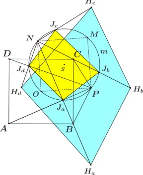
Property 2. The pointsO,P,Ja,Jb,Jc andJd lie on a circle. In particular, the quadrangle JaJbJcJd is cyclic.
We can say more about the circlemwhich appears in the Property 2. It is the circumcircle of the negatively oriented square P ON M built on the segment P O.
Hence, if |P O|=δ, then the radius of the circlemis δ√22 (see Figure 2).
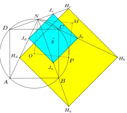
The third property describes the following surprising connection of the quad- ranglesHaHbHcHd andJaJbJcJd(see Figure 3).
Property 3. The linesHaJa,HbJb,HcJc and HdJd intersect in the pointN and go through the points B,C,D andA, respectively.
Now one can wonder when is the quadrangleHaHbHcHd cyclic and when will the quadrangleJaJbJcJdhave perpendicular diagonalsJaJcandJbJd. The answers give the following two theorems.
A B D C
O
Ja
Jb Jc
Jd
S
P
Figure 2: The cyclic quadrangleJaJbJcJd.
Theorem 1.1. The quadrangle HaHbHcHd is cyclic if and only if the point P is either on the line AC, on the line BD or on the circumcircle k of the square ABCD.
Theorem 1.2. In the quadrangle JaJbJcJd the linesJaJc andJbJd are perpendic- ular if and only if the pointP is either on the line AC, on the lineBD or on the circumcirclek of the square ABCD.
More precisely, Ha =Hc and/or Hb=Hd if and only if P is either on the line AC or on the lineBD. Hence, the first two parts of the locus from Theorems 1.1 and 1.2 correspond to the case when the quadrangle HaHbHcHd degenerates to a segment or a point and either Ja=Jc or Jb=Jd. The role of the third part (the circumcirclek) is explained better by the following statement: IfP is on the circumcirclek, then
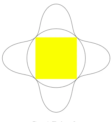
(a)HaHbHcHd is a square of side equal to the diagonals ofABCD with P as the center whose diagonalsHaHc andHbHd are parallel to the linesBC andAB, (b)JaJbJcJdis also a square of side equal to the half of the diagonals ofABCD, (c) JaJbJcJd and HaHbHcHd are related by the homothety h(N,2) where N is the vertex of the square on the segmentP O (see Figure 4).
A B D C
O
Ha
Hb Hc
Hd
Ja
Jb Jc
Jd S
P
N M
m
Figure 3: The linesHaJa,HbJb,HcJc andHdJd concur in the pointN.
An interesting path is to explore how the areas of the quadranglesHaHbHcHd
and JaJbJcJd compare to the area Ω of the square ABCD. We define the area
|W XY Z| of the quadrangle W XY Z as the sum |W XY|+|W Y Z| of (oriented) areas of the trianglesW XY andW Y Z.
For every real numberm letPm and Qm denote the loci of all points P such that |HaHbHcHd|=mΩand|JaJbJcJd|=mΩ, respectively.
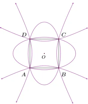
Theorem 1.3. For m <0, m= 0, 0< m <2, m= 2 and m >2 the set Pm is the union of two hyperbolas, the union of lines AC and BD, the empty set, the circumcirclek of the squareABCD, and the union of two ellipsis, respectively. If the axes of one conic areϕandψ then the axes of the other areψ andϕ.
The Figures 5 and 6 show the setsPmfor m=−1 andm= 3 and the setQ1 together with the square ABCD. Notice thatQ1 2
2 is the union of the circumcircle k of the square ABCD and a symmetric curve of order six that touchesk in the vertices of the square.
Let us conclude this description of our results with some comments on what else one can do with this approach. Instead of orthocenters we can consider other central points of the triangle (like the centroid, the circumcenter, the center of the nine-point circle – see the references [3] and [4] for the list of more than thou-