TURBO-20-1342 Daku 1
Experiments-Based Preliminary Design Guidelines for Consideration of Profile Vortex Shedding from Low-Speed Axial Fan
Blades
Gábor Daku*, first author1
Department of Fluid Mechanics, Faculty of Mechanical Engineering, Budapest University of Technology and Economics
Bertalan Lajos u. 4 – 6., H-1111 Budapest, Hungary daku@ara.bme.hu
János Vad, second author
Department of Fluid Mechanics, Faculty of Mechanical Engineering, Budapest University of Technology and Economics
Bertalan Lajos u. 4 – 6., H-1111 Budapest, Hungary vad@ara.bme.hu
ASME Membership
ABSTRACT
The paper presents hot wire measurements in a wind tunnel, close downstream of basic models of blade sections being representative for low-speed, low-Reynolds-number axial fans, in order to explore the signatures of vortex shedding (VS) from the blade profiles. Using the Rankine-type vortex approach, an analytical model was developed on the velocity fluctuation represented by the vortex streets, as an aid in evaluating the experimental data. The signatures of profile VS were distinguished from blunt-trailing-edge VS based on Strouhal numbers obtained from the measurements in a case-specific manner. Utilizing the experimental results, the semi-empirical model available in the literature for predicting the frequency of profile VS was extended to low-speed axial fan applications. On this basis, quantitative guidelines were developed for consideration of profile VS in preliminary design of axial fans in moderation of VS-induced blade vibration and noise emission.
1 Corresponding author.
TURBO-20-1342 Daku 2 INTRODUCTION AND OBJECTIVES
The subject of the present paper is periodic shedding of coherent vortices over the lifting surface of profiles of low-speed axial flow fan rotor blades. This phenomenon, termed herein profile vortex shedding (PVS), is well distinguished from trailing-edge- bluntness vortex shedding [1], occurring past the blunt trailing edge (TE) of the blade, acting as the aft portion of a bluff body. In the aforementioned reference, PVS is referred to as laminar-boundary-layer vortex shedding. The reason for this nomenclature is that a precondition for PVS is the existence of laminar boundary layer over a significant portion of at least one side of a blade profile. The occurrence of PVS is related to Tolmien-Schlichting instability waves originating in the laminar boundary layer upstream of the TE. As discussed in [2], PVS may occur even if the boundary layer is turbulent but the Reynolds number is moderate, i.e. Re ≤ 1.5·105. In this case, the initially laminar suction side boundary layer, being separated near the leading edge, is subjected to laminar-to-turbulent transition, and reattaches upstream of mid-chord position. The generality of occurrence of vortex shedding related to either laminar or turbulent boundary layers makes the use of the generalized term PVS reasonable. The substantially different mechanisms of TE-bluntness vortex shedding and PVS manifest themselves in distinct scaling definitions and values of Strouhal numbers, specified below. Some quantities related to the Strouhal number definitions are illustrated in Fig.
1.
For TE-bluntness vortex shedding [3]:
StTE = fTE⋅dTE / U0 ≅ 0.20 (1)
TURBO-20-1342 Daku 3 For PVS [2, 4-5]:
St* = fPVS⋅b / U0 ≅ 0.16 (2)
In [2, 4-5], St* is referred to as universal Strouhal number, suggesting that its value of ≅ 0.16 is considered to be universally valid for various profile geometries. The validity of this consideration has been limited in these references by the fact that detailed fluid mechanics measurements on fPVS and b are available only for relatively thick, symmetrical airfoil profiles, out of the NACA-00 series. Such profiles are unusual for rotor blades of low-speed axial fans. No detailed fluid mechanics measurement data are available in the literature on the PVS phenomenon related to asymmetrical blade profiles relevant to low-speed axial fans, such as cambered plate, or asymmetrical airfoils. Therefore, the presently available semi-empirical model for estimation of PVS frequency, based on St*, [2, 4-5], has not yet been extended empirically to low-speed axial fan applications.
Fig. 1 Illustration for vortex shedding
The critical overview of the effects of PVS is of engineering relevance from two perspectives: noise and vibration. PVS noise is characteristic for ventilating fans [6-8]. In [8], it is stated that noise generated by vortex shedding is the primary noise source for small fans. Furthermore, classifying the sources of self-noise for fan blades [1, 9], it is concluded herein that PVS is the only aeroacoustics noise source that may generate periodic, spatially coherent pressure fluctuations over a remarkable portion of the blade
TURBO-20-1342 Daku 4 surfaces. The result is a periodically fluctuating force normal to the chord of the
elemental blade sections. In order to illustrate the magnitude of fluctuating blade force due to PVS, the case study in [5] is referred to. In this case study, a force fluctuation in the order of magnitude of ± 10 percent of the temporal mean blade lift coefficient, due to PVS, is reported for an airfoil section. Such force leads to a fluctuating bending moment that may cause vibration of rotor blades of moderate inertia, i.e. thin plate blades (occasionally made of polymer material), being frequently used for low-speed fans. In [10], the accelerometer installed on the airfoil indicated vortex-induced vibration, the dominant frequency spike of which coincided with the far-field tone frequency.
The dominant frequency of PVS is a key factor in judging its impact from the perspectives of aeroacoustics as well as structural mechanics. On one hand, if the dominant frequency of PVS coincides with an eigenfrequency of the blade, resonance may occur, which may cause the axial fan rotor to imbalance / break down. On the other hand, having this frequency close to the plateau of the A-weighting graph [11-12]
increases the probability that the PVS noise approaches a level of audibility that might cause irritation to a human.
From practical point of view, it is desirable to formulate approximate quantitative guidelines, in closed algebraic form for straightforward treatment, providing a means for consideration of PVS in preliminary blade design. With use of such guidelines, the main trends can be briefly characterized, and the blade parameters can systematically be harmonized, for achieving the following, twofold goals. i) Prevent shedding of extensive,
TURBO-20-1342 Daku 5 coherent vortices of uniform frequency from a significant portion of blade span, being
adverse in terms of mechanical excitation of the blades. ii) Moderate the adverse acoustic effect of PVS from the viewpoint of human audition, being especially important in the case of low-speed ventilating fans operating in the vicinity of humans. The literature lacks in providing such brief design guidelines in blade aerodynamics as well as in aeroacoustics.
The experiments in the literature on PVS regard isolated rectilinear blade or wing models. Based on [1, 3, 6, 8-9], these studies can be considered as approximate representations of two-dimensional (2D) flow in low-solidity annular cascades in a rotor.
For calculation of case-specific values of St* defined in Eq. (2), fPVS as well as b are to be obtained from the measurements. For determining b, the vortex centers within the pair of rows of shed vortices are to be localized. In the experiments in [2, 4, 13-15], the maxima of root-mean-square (RMS) of velocity fluctuation were considered as loci of the axes of shed vortices in vortex rows.
Hot wire measurements are often involved in the vortex shedding studies [2, 4, 15].
The literature appears to be contradictory in the measurement and evaluation methodology, with special regard to vortex center detection. The following questions arise. i) What type of hot wire measurement technique is to be applied – single- component (1D), or two-component (2D)? ii) The RMS of which measured velocity component is to be evaluated – RMS(v′) measured by a 1D probe, or either RMS(v′X) or RMS(v′Y) measured by a 2D probe?
TURBO-20-1342 Daku 6 Reference [4] suggests the necessity of applying a 2D hot wire experiment for PVS
detection. In [4], the vortex center is represented by a peak in the RMS(v′Y) distribution, and spectra of RMS(v′Y) are reported. It is concluded in [4] that the authors in [16] failed to point out the PVS phenomenon probably due to the limitation represented by the 1D hot wire anemometer technique used in [16]. In [2], RMS(v′X) has been evaluated, and b has been determined as the transversal distance between two well-distinguished peaks in the RMS(v′X) distribution. Similar to [4], spectra of RMS(v′Y) are reported in [2]. In [15], 1D hot wire studies are presented. Spatial and spectral distributions of RMS(v′) are reported. The streamwise development of location of maximum of RMS(v′) is considered as indicator of vortex trajectory.
The above overview demonstrates the lack of theoretical confirmation of relationship between the location of vortex center in a shed vortex row and the spatial distribution of RMS of fluctuating velocity.
In the view of the aforementioned lack in the open literature, the paper sets the following engineering tasks of novelty content.
a) Elaboration and experimental validation of a new analytical model to support the reliable examination and quantification of the PVS phenomenon. This model serves for theoretical confirmation of reliability of 1D hot wire measurements reported herein by the authors in investigation of vortex shedding.
b) Extension of the experimental database in the literature on PVS, using hot wire measurement data taken on representative asymmetrical profiles used for low-speed
TURBO-20-1342 Daku 7 axial fan rotor blades. Evaluation of the measurements using the analytical model
outlined in Point a).
c) Extension of the semi-empirical model for estimation of PVS frequency, based on St*, to representative low-speed axial fan blade profiles, by utilizing the measurement data outlined in Point b).
d) Elaboration of new preliminary blade design guidelines using the extended semi- empirical model outlined in Point c) for moderation of vibration propensity of low- speed axial fan rotor blades due to PVS.
e) Using the model of Point c), formulation of a preliminary design guideline for moderation of PVS noise from the aspect of audibility by humans.
EXPERIMENTAL TECHNIQUE
The experiments were performed in the Blackbird-2 open-loop wind tunnel, outlined in Fig. 2. The facility is operated at the Department of Fluid Mechanics, Faculty of Mechanical Engineering, Budapest University of Technology and Economics. The 1 m- long test section of the wind tunnel has a height of 1 m and spanwise extension of 0.15 m. The freestream velocity can be varied up to 21 m/s, and was monitored using a calibrated Pitot-static tube and a pressure transducer of type Setra 239, calibrated to a certified Betz micromanometer. The maximum of the free-stream turbulence intensity was ≈ 1% at the middle of the test section. The air temperature was measured using a GMH 3710 high precision digital thermometer. Further details of the wind tunnel technique are reported in [17].
TURBO-20-1342 Daku 8 Fig. 2 Experimental setup. (1) Motor, (2) Frequency converter, (3) Radial fan, (4) Inlet
bellmouth, (5) Guide vanes, (6) Flexible connector, (7) Split diffuser, (8) Honeycomb, (9) Turbulence reduction screens, (10) Transition element, (11) Test section.
The isolated, rectilinear basic models of low-speed axial fan blades of span of S = 150 mm were inserted between the endwalls of the test section. The gaps between the profile tips and the endwalls were minimized, in accordance with the instructions in [18]. The angle of attack α was set with use of a manual protractor.
The flow velocity measurements in the near-wake region were carried out using Constant Temperature Anemometry (CTA), by means of a Dantec 1D hot wire probe, connected to a DISA 55M01 type CTA bridge. The wire diameter is 5µm. The wire was aligned parallel to the span of the blade models. The probe was mounted on a Cartesian automated traversing system, allowing traverses in streamwise (X) and transversal (Y) direction. The origin of the X-Y coordinate system corresponds to the TE of each blade profile, as illustrated in Fig. 3. The probe was traversed along the Y direction at a distance of 0.10c downstream of the TE.
Pressure, temperature, and velocity data were acquired and processed using the in- house developed Pressure & Force measurement software, through an NI BNC-2110
TURBO-20-1342 Daku 9 shielded connector block and an NI PCI-6036E data acquisition card. The spectral
analysis of the hot wire signals was carried out using Fast Fourier Transformation (FFT).
The absolute errors of the measured and derived quantities being relevant in the discussion in the paper are given in Table 1. The estimation of the absolute errors followed the methodology in [19]. The errors for the hot wire-measured velocity data were estimated on the basis of [20], considered as a departmental preliminary study to the application of hot wire anemometry to flow phenomena related to axial flow fans.
Fig. 3 Coordinate systems
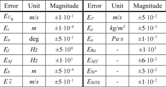
Table 1 Estimation of averaged absolute errors
Error Unit Magnitude Error Unit Magnitude EU0 m/s ±1⋅10-1 Ev′ m/s ±5⋅10-2
Ec m ±1⋅10-4 Eρ kg/m3 ±5⋅10-3
Eα deg ±5⋅10-1 Eμ Pa·s ±1⋅10-7
Ef Hz ±5⋅100 ERe - ±1⋅103
EΔf Hz ±1⋅101 EΔf/f - ±6⋅10-2
Eb m ±5⋅10-4 ESt* - ±3⋅10-2
Ev m/s ±5⋅10-1 EStTE - ±1⋅10-2
The measurements intend to represent elemental fan blade sections in a 2D flow approximation. This corresponds to the preliminary aerodynamic design approach of cylindrical stream tubes through the blading [9]. The 2D view is of importance also in aeroacoustic modeling of the blade sections. Acoustic measurement data obtained for 2D blade sections can be adapted to rotating blades, by means of a spanwise segment
TURBO-20-1342 Daku 10 splitting [3]. The 2D approximation was fulfilled by means of the following considerations. i) The experimental setup corresponds geometrically and aerodynamically to the 2D approximation presented in [18]. ii) The hot-wire probe was set to midspan position. The resultant symmetry condition was considered to eliminate the impact of the spanwise velocity component, if any, on the measurements. iii) Since each model has a chord length of c = 100 mm, the aspect ratio is S/c = 1.50, being in correspondence with the wind tunnel studies in [18]. The studies in [21] reveal that, even in the case of such low aspect ratio, the vortex shedding frequency fairly approximates the frequency valid for a 2D case.
CASE STUDIES
Considered as representative asymmetrical blade profiles in low-speed axial fan applications, a circular-arc cambered plate with 8 % relative camber, and a RAF6-E airfoil profile, were studied. In addition, as a fluid mechanics reference case, a flat plate was also involved. From this point onwards, the three studied profiles are shortly termed as flat, cambered, and airfoil profile. Within the family of circular-arc cambered plates, the 8 % cambered profile provides a nearly maximum lift-to-drag ratio, enabling preliminary fan design for high efficiency [9]. For both of the cambered and the airfoil profiles, the lift coefficient CL at maximum lift-to-drag ratio is ≈ 1 [22], and therefore, they are competitive from preliminary fan design point of view. As [18] suggests, at Rec < 105, cambered plates tend to become aerodynamically more favorable – i.e. increased CL, decreased CD – than airfoils. Therefore, the range surrounding Rec ≈ 105 deserves a special attention in low-speed fan design. In order to incorporate such range, and to fit
TURBO-20-1342 Daku 11 to the Re-ranges investigated in [18], the experiments presented herein were carried
out at three different Reynolds numbers: Rec = 0.6·105; 1.0·105; and 1.4·105, corresponding to U0 = 9.0 m/s; 15.0 m/s; and 21.0 m/s, respectively. It is noted that studies within this Re-range add to the classic fan design literature proposing higher Re values, i.e. above the limit of Rec = 1.5·105 [9], for fan operation at reasonably high efficiency. It was intended to stay far away from the stalled state but to consider test cases in the surroundings of maximum lift-to-drag ratio [22]. Therefore, studies for angles of attack of α = 0°; 2°; 4°; and 6° were carried out. All of the aforementioned choices fit to preliminary studies in [17, 23].
The leading and trailing edges are left blunt for the flat and cambered profile, representing a simplification in manufacturing of low-speed fans [24]. The flat, cambered, and airfoil profiles are shown in Fig. 4. Table 2 contains the geometrical data of the rectilinear blade models.
Fig. 4 Profiles under investigation. Flat (top), cambered (middle), airfoil (bottom).
TURBO-20-1342 Daku 12 Table 2 Geometrical data of the blade models
MEASURED FLOW DETAILS: EXAMPLES
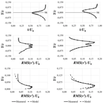
Out of the hot wire measurement campaign carried out on the three models at the three Reynolds numbers and the four angles of attack, Fig. 5 presents data on two scenarios as illustrative examples, both being valid for the operating condition of Rec = 0.6·105 at α = 0°. In the left column, data on the flat profile are presented. The right column shows data on the airfoil. The data of velocity dimension, specified on the horizontal axes, are normalized by U0. The data on the Y-wise position, being zero at the mid-point of TE location, and specified along the vertical axes, are normalized by c. At the top, the temporal mean velocity distributions are presented. In the middle row, the transversal distributions of RMS of fluctuating velocity are shown, in which double peaks can be observed. For the flat profile, some asymmetry appears in the distributions, with respect to the Y = 0 plane. This is dedicated to the uncertainty of the adjustment of α = 0°, within the range specified in Table 1. A primary intention of processing the measurement data is to determine the b transversal distance between the vortex rows, serving as input for calculating St* in Eq. (2). Following [2, 4, 13-15], one may intuitively presume that the double peaks correspond to the pair of rows of shed vortices, and the Y-wise distance between the two maxima equals b. However, it is to be kept in mind that a 1D hot wire instrument was used herein, providing RMS(v′). Considering the
Profile c [mm] S [mm] z [mm] d [mm]
Flat 100 150 2.5 0
Cambered 100 150 2.1 8
Airfoil 100 150 10.0* 5
*Maximum thickness
TURBO-20-1342 Daku 13 peaks of RMS(v′) as vortex centers may oppose the views in [2] and [4], localizing the
vortex centers to peaks of RMS(v′X) and RMS(v′Y), respectively, and stating the necessity of use of 2D hot wire anemometry. In order to provide a theoretical confirmation of reliability of 1D hot wire measurements in quantifying b in the present studies, an analytical model has been developed.
Fig. 5 Illustrative examples for the hot wire measurement results. Rec = 0.6·105, α = 0°.
Left column: flat. Right column: airfoil. Temporal mean velocity (top) and fluctuating velocity RMS (middle) distributions. Bottom: enlarged sections of the diagrams in the
middle row.
ANALYTICAL MODEL
The analytical model described herein, expressing the velocity fluctuation represented by the shed vortices, relies on the Rankine-type combined vortex model.
The Rankine-type vortex modeling approach is widely used for modeling the vortex
TURBO-20-1342 Daku 14 shedding phenomenon related to turbomachinery blades [25-27]. According to the model, a vortex represents the following vV(r) “vortex velocity” distribution, observed from the coordinate system having an origin bound to the vortex center, having [x, y]
axes being parallel with the [X, Y] axes, and translating together with the vortex at a velocity of UV in streamwise direction – as illustrated in Fig. 3:
Vortex core: r ≤ RV; vV(r) = r⋅ω (3a)
Whirl region: r > RV; vV(r) = RV2 ⋅ω / r (3b) The profiles produce lift, and thus, deflect the flow. Therefore, the streamwise direction followed by the shed vortices differs from the X-direction. However, considering the moderate α and CL values, the direction of the vortex rows is approximated for simplicity as the X-direction (Fig. 3). This simplification has insignificant impact on the results presented herein. Based on the diagrams at the top of Fig. 5, the following brief estimation is made on the orders of magnitude of ω and RV, being generally valid for the studies presented herein, in order to provide quantitative guidelines for setting of model parameters. The thickness of the boundary layer at the TE is δ ≈0.1c = 10 mm. According to the no-slip condition, the velocity is zero at the blade surface. Accordingly, considering the blade position as center of rotation, and viewing U0 = 9.0 m/s – set for Rec = 0.6·105 in each experiment – as a fictitious circumferential velocity of solid body rotation of ω angular speed at a radius of δ, reads ω ≈ 900 1/s. Considering the boundary layer of δ ≈ 10 mm as a flow domain enveloping
TURBO-20-1342 Daku 15 the shed vortices of core diameter of 2RV, reads RV ≈ 5 mm. On this basis, the orders of
magnitudes for various operating conditions are as follows:
Order of ω magnitude: 103 1/s (4a)
Order of RV magnitude: 10-3 m (4b)
The vortex velocity of Eqs. (3a) and (3b) consists of the following x-wise and y-wise components:
vVx = vV⋅y / r (5a)
vVy = – vV⋅x / r (5b)
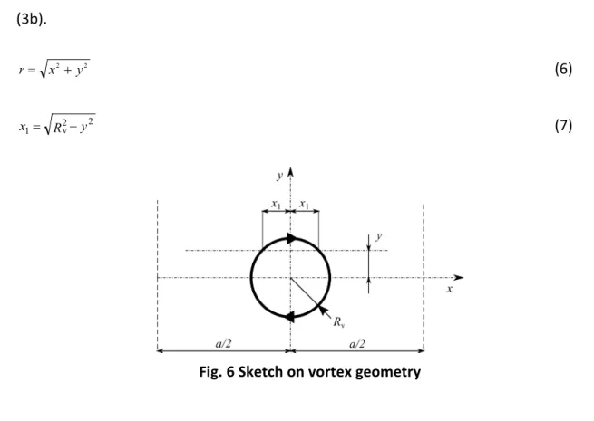
Figure 6 illustrates the following relationships between the coordinates, at any fixed y value. x1 serves for making a distinction between the validity ranges of Eqs. (3a) and (3b).
2
2 y
x
r= + (6)
2 2 v
1 R y
x = − (7)
Fig. 6 Sketch on vortex geometry
TURBO-20-1342 Daku 16 Any quantity q is composed of temporal mean and fluctuating components:
' q q
q= + (8)
Where the temporal mean value is considered as an integral mean value over an appropriate interval T:
= t+T∫
tqdt
q T1· (9)
Substituting Eq. (8) into Eq. (9) reads that the temporal mean value of the fluctuating component is to be zero:
0 '≡
q (10)
When modeling the velocity fluctuation v′ in the flow field, such fluctuation was regarded exclusively as consequence of the shed vortices, i.e. no velocity fluctuation was considered in absence of the vortices. It is considered that the vortex street travels at a constant velocity UV. The vortices follow each other within the row at a distance of a (conf. Fig. 1). Thus, the velocity field represented by the vortices in a row is periodic, with a length of period of a, as indicated in Fig. 6 with dashed y-wise lines at the edge.
For calculating the velocity fluctuation, it is therefore sufficient to take a single period of length a into consideration. The relationships 1/T = UV/a and dt = dx/UV are applied. On the basis of all above, the temporal integration in Eq. (9) can be transformed to spatial integration. The temporal mean value of q(x,y), for any fixed y, can be expressed as follows:
= ∫
= ∫
−
+ /2
2 / ( , ) 1·
1· )
( a
a T
t
t q x y dx
dt a T q y
q (11)
TURBO-20-1342 Daku 17 The Y-wise component of velocity fluctuation can be modeled as follows, with use of
Eq. (5b):
v′Y (x,y) = vVy (x,y) (12)
The fluctuating components must fulfill the condition in Eq. (10). In the case of Eq.
(12), this condition is fulfilled, since the x-wise range of integration is ± a/2, conf. Eq.
(5b). In order to fulfill the condition of Eq. (10) also for the x-wise component of velocity fluctuation, the following modeling consideration is to be made, taking Eqs. (5a) and (11) as a basis:
) ( ) , ( ) ,
( V V
X x y v x y v y
v′ = x − x (13)
With use of Eqs. (12) and (13), v′ is expressed as follows:
( ) ( )v 2 v 2
v′= ′X + ′Y (14)
In order to obtain the analytical description of velocity fluctuations, Eqs. (3a), (3b), (5a), (5b), (6), (7), (11), (12), (13), and (14) are to be used in an organized manner. For any fixed y position, the square of Eqs. (12) to (14) can be taken. Then, the temporal mean of these squares can be expressed with use of integration in Eq. (11). Finally, the square root of the result is to be calculated, thus obtaining the RMS values, being dependent on y. This procedure therefore results in the modeled y-wise distributions of RMS(v′X), RMS(v′Y), and RMS(v′), related to vortex shedding. As illustrated in Figs. 3 and 6, the vortex center is defined at the position of y = 0. On this basis, the applicability of the aforementioned RMS distributions in localization of vortex center can be judged.
TURBO-20-1342 Daku 18 UTILIZATION OF THE ANALYTICAL MODEL
The analytical model has been applied and evaluated for various parameter settings of RV and ω, in comparison to the measured RMS(v′) distributions. The parameters were set systematically within the estimated ranges of order of magnitude – see the comments below Eqs. (3). In what follows, the application and evaluation of the analytical model is discussed.
The modeled RMS(v′) distribution shows local maxima at the boundaries of the vortex core, i.e. at y = ± RV. Relative to these maxima, RMS(v′) exhibits a “dip”
(reduction) at y = 0. However, this dip is slight, being in the order of magnitude of Ev′. It is also to be kept in mind that the Rankine model is the simplest approach for a vortex with a viscous core. It has been chosen at the present phase of research for its easiest analytical treatment. The vV(r) distribution represented by Eqs. (3a)(3b) has an acute peak at RV. By applying “blending” in the vV(r) distribution in the vicinity of RV, incorporating more realistic vortex models published in the literature [28-29], the aforementioned dip tends to diminish, and the RMS(v′) distribution tends to exhibit a maximum at y = 0, i.e. at the vortex center location. Ongoing research by the authors focuses on such improvement of the vortex model, for a more advanced evaluation of the hot wire results. The comments above allow for the following conclusion. In absence of 2D hot wire measurements, and relying on a 1D hot wire technique, the measured RMS(v′) distribution provides a reasonable compromise in searching for the vortex center. First, the locus of vortex center is approximated at the local maximum of RMS(v′). At this location, the Fourier spectrum of RMS(v′) is to be analyzed, and the
TURBO-20-1342 Daku 19 distinct frequency peak f dedicated to vortex shedding is to be identified. Then, along
the Y coordinate in the vicinity of the RMS(v′) maximum location, the RMS(v′) amplitudes at f are to be examined. The Y location at which the RMS(v′) amplitude at f reaches its maximum is to be considered as the locus of vortex center.
In order to illustrate this vortex center detection process, the diagrams in the bottom row of Fig. 5 are to be observed. They present enlarged views of the upper peaks in the RMS(v′) distributions in the middle row of diagrams. The solid and dashed lines correspond to the measured and modeled RMS(v′) distributions, respectively. For the modeled distributions, the parameter settings of RV and ω were systematically modified within the estimated ranges of orders of magnitude, in order to provide best fitting to the measurements. The modeled RMS(v′) distributions shown in Fig. 5 correspond to the following settings. For the flat profile, RV = 0.80 mm and ω = 4000 1/s.
For the airfoil profile, RV = 0.96 mm and ω = 6000 1/s. A fair agreement can be observed between the measured and modeled RMS(v′) distributions, demonstrating the reasonability of the applied Rankine model at the present phase of approach. The discrepancy between the measured and modeled data is mainly dedicated to the fact that the measured RMS(v′) data also incorporate the turbulent fluctuations being present in the flow field but disregarded in the vortex model.
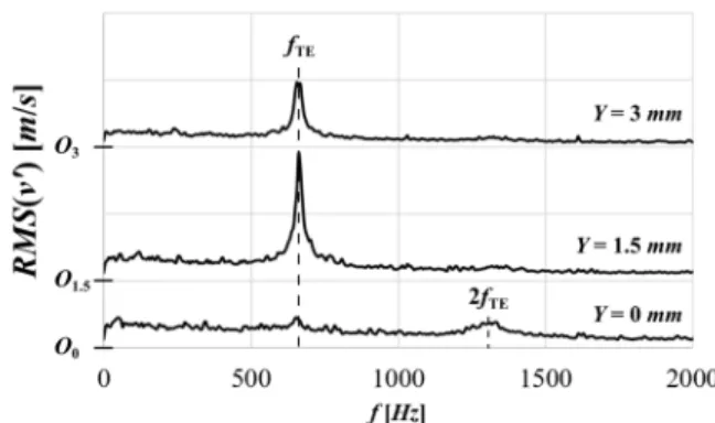
Figures 7 and 8 present the Fourier spectra of measured RMS(v′), corresponding to the case studies in the bottom row of Fig. 5, for various Y locations taken as examples.
The vertical scaling unit is 0.2 m/s. As commented in the figure captions, the horizontal axes related to the individual graphs are shifted for better visibility. For the flat plate –
TURBO-20-1342 Daku 20 Fig. 7 –, at maximum RMS(v′) in Fig. 5, f = fTE has been identified as the dominant peak
corresponding to vortex shedding. The figure illustrates that this frequency peak invariably characterizes the flow field at various Y positions. Furthermore, it is characteristic for both the upper and lower peaks in the RMS(v′) distribution along Y.
Illustrated by Fig. 7, the Y = 1.5 mm position, assigned to the maximum amplitude in the spectrum, has been considered as the location of vortex center in the upper vortex row.
This peak position has been marked with a small “+” symbol in the diagram in the bottom row of Fig. 5. The position of this symbol fits fairly well to the centerline (corresponding to y = 0) of the modeled RMS(v′) distribution, indicating that it is a reliable representation of the vortex center. The same process can be followed for the airfoil profile – Fig. 8 –, considering f = fPVS as dominant frequency, exhibiting a peak amplitude in the spectrum at Y = 5 mm, regarded therefore as locus of vortex center, as indicated at the bottom of Fig. 5 with a small “+” symbol.
The same process applies for the localization of the center of the lower vortex row.
As the difference between the Y positions assigned to the vortex centers, b can be determined.
The above discussion confirmed the appropriateness of using a 1D hot wire instrument herein, providing RMS(v′), in vortex center detection. This confirmation is supported by Ref. [15].
The apparent contradiction in the literature [2, 4, 15-16], discussed formerly, deserves additional comments on the analytically modeled RMS(v′Y) and RMS(v′X) distributions. The modeled RMS(v′Y) distribution along the y coordinate exhibits a
TURBO-20-1342 Daku 21 maximum at y = 0, i.e. at the vortex center location. This is in accordance with the view
in [4] that the vortex centers can be localized by finding the maxima in the RMS(v′Y) distribution. The modeled RMS(v′X) is zero at y = 0 but reaches its maximum at y = ± RV. Therefore, the boundaries of the vortex core can be mapped also on the basis of RMS(v′X), giving an implicit representation of the vortex center at mid position.
Therefore, RMS(v′X) may also serve as basis for localization of vortex center, being in accordance with [2]. Based on the above, it is concluded that either RMS(v′) or RMS(v′Y) or RMS(v′X) can be used in determination of locus of vortex center, with involvement of an appropriate, theoretically established evaluation methodology.
Figures 7 and 8 draw the attention to a phenomenon termed herein frequency duality. In addition to the dominant peaks of fTE and fPVS, furher peaks, although considerably weaker, appear at 2⋅fTE and 2⋅fPVS. These additional peaks tend to amplify with decreasing Y, i.e. toward the mid position between the two vortex rows. The frequency duality is explained in Fig. 9. If the hot wire is faced with a single vortex row, indicated in a position of HW1 in the figure, the detected dominant frequency will be determined by the repetition of vortices passing the sensor with periodicity of a. In this case, the dominant frequency is expressed as follows:
f = UV/a (15a)
TURBO-20-1342 Daku 22 Fig. 7 Flat plate, Rec = 0.6·105, α = 0°. Measured RMS(v′) spectra for various Y
coordinates. Vertical scaling unit: 0.2 m/s. The horizontal axes are shifted for better visibility. The origins are indicated on the left using “O” symbols with indices equal to
the related Y position.
Fig. 8 Airfoil, Rec = 0.6·105, α = 0°. Measured RMS(v′) spectra for various Y coordinates.
Vertical scaling unit: 0.2 m/s. The horizontal axes are shifted for better visibility. The origins are indicated on the left using “O” symbols with indices equal to the related Y
position.
If the sensor is traversed toward the mid position between the two vortex rows, indicated in the figure in a position of HW2, the detected fluctuations will although be weaker, however, the fluctuations represented by both vortex rows are sensed. Since the vortices in both rows are of periodicity of a but a phase shift corresponding to a/2
TURBO-20-1342 Daku 23 occurs between the rows, the sensor will detect a repetition of fluctuation with
periodicity of a/2. Therefore, the dominant frequency is obtained as
UV/(a/2) = 2⋅f (15b)
The frequency duality appears in the experiments in [4] (Figs. 6 and 16b). It can be traced not only in fluid mechanics measurements but also in aeroacoustics related to vortex shedding. The sound pressure spectra in the following references suggest the presence of a peak of 2⋅f in addition to the dominant peak of f, although being ≈ 15÷20 dB weaker than the dominant one: [1](Figs. 83 and 84); [10](Fig. 3); [30](Fig. 4). The Phased Array Microphone studies in [31] also confirm the frequency duality phenomenon.
Fig. 9 Scheme for explanation of frequency duality
VORTEX SHEDDING: RESULTS AND DISCUSSION
The hot wire data were systematically evaluated in accordance with the considerations outlined above. The occurrence of vortex shedding was considered to be confirmed only in cases for which two distinct peaks were detected in the Y-wise
TURBO-20-1342 Daku 24 distribution of the experiment-based RMS(v′) data, with identical dominant frequencies
f. The experimental data are presented in Tables 3 to 6.
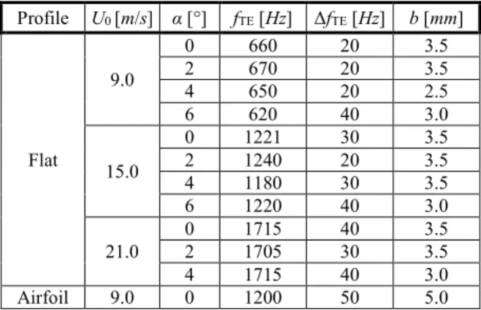
In Tables 3 and 4, those experimental data are collected for which the occurrence of TE-bluntness vortex shedding has been concluded, in accordance with the following considerations. In Table 3, the quantities with dimensions are summarized. Δf represents the half-width of the dominant frequency peak, i.e. the average width of the frequency bands at half of the maximum amplitudes of the two distinct peaks related to shed vortices on the suction and pressure sides. In Table 4, dimensionless quantities are derived using the data of Table 3 for further evaluation. For the airfoil profile, dTE is 1.6 mm, considered as twice the TE radius [22]. It is conspicuous in Table 3 that the detected b values provide an approximate upper estimation of the z data specified in Table 2 for the flat plate, i.e. 2.5 mm, being equal to the TE thickness in this case. This suggests intuitively that the detected vortex shedding phenomenon is related to TE- bluntness vortex shedding.
Table 4 provides data for two types of Strouhal number definitions, in order to support the clear distinction between the two types of vortex shedding phenomena assigned to Eqs. (1) and (2). The StTE definition in the table corresponds to Eq. (1). The StTE data calculated in Table 4 well approximate the StTE ≅ 0.20 value specified in Eq. (1), exhibiting an average value of 0.19. In evaluating these data, it is to be taken into account that EStTE = ± 0.01, according to Table 1. The StTE data serve as a confirmation of the occurrence of TE-bluntness vortex shedding in the cases presented in Table 4.
Accordingly, the frequency data in Tables 3 to 4 are equipped with the index TE. The
TURBO-20-1342 Daku 25 other Strouhal number definition in the table, fTE⋅b/U0, would represent St*=fPVS⋅b/U0 ≅
0.16, according to Eq. (2), if the vortex shedding phenomenon presented in the table would be a PVS phenomenon. As the table suggests, the data of fTE⋅b/U0 show increased variance in comparison to data in the StTE column, about the average value of 0.26. In most cases, these data are significantly different from 0.16 expected in the case of PVS.
This supports the reasonability of excluding the occurrence of PVS in these cases.
In the sole case of TE-bluntness vortex shedding detected for the airfoil profile, conf.
Table 4, the related fTE peak is presented in Fig. 8. This peak is well-separated from the other two peaks dedicated to PVS with consideration of frequency duality. For the flat plate, the fTE and 2⋅fTE peaks, corresponding to the frequency duality phenomenon, are illustrated in the example in Fig. 7.
As Tables 3 and 4 suggest for the flat plate, no evidence was found for TE-bluntness vortex shedding at the data couple of maximum Rec of 1.4·105 and maximum α of 6°.
Furthermore, for the airfoil, no evidence was found for TE-bluntness vortex shedding for Rec > 0.6·105 and α > 0°. These observations allow for the qualitative statement that TE- bluntness vortex shedding tends to occur toward moderate Rec and / or α values.
TURBO-20-1342 Daku 26 Table 3 Experimental data on TE-bluntness vortex shedding: quantities with
dimensions
Profile U0 [m/s] α [°] fTE [Hz] ΔfTE [Hz] b [mm]
Flat
9.0
0 660 20 3.5
2 670 20 3.5
4 650 20 2.5
6 620 40 3.0
15.0
0 1221 30 3.5
2 1240 20 3.5
4 1180 30 3.5
6 1220 40 3.0
21.0 0 1715 40 3.5
2 1705 30 3.5
4 1715 40 3.0
Airfoil 9.0 0 1200 50 5.0
Table 4 Experimental data on TE-bluntness vortex shedding: dimensionless quantities
Profile Rec α [°] ΔfTE/fTE fTE⋅b/U0 StTE
Flat
0.6·105
0 3.0 % 0.26 0.18
2 3.0 % 0.26 0.19
4 3.0 % 0.18 0.18
6 6.5 % 0.21 0.17
1.0·105
0 2.5 % 0.28 0.20
2 1.6 % 0.28 0.21
4 2.5 % 0.28 0.20
6 3.3 % 0.25 0.20
1.4·105 0 2.3 % 0.29 0.20
2 1.8 % 0.29 0.20
4 2.3 % 0.25 0.20
Airfoil 0.6·105 0 2.6 % 0.22 0.20 Average: 0.26 0.19
Tables 5 and 6 summarize the data considered to be related to the PVS phenomenon. The data, their representation and evaluation are organized in a manner similar to those related to Tables 3 and 4.
The St* data in Table 6, corresponding to Eq. (2), fairly well approximate the St* ≅ 0.16 value in most cases, providing an average value of 0.19. This is a confirmation of the occurrence of PVS in the cases presented in Table 6. Accordingly, the frequency data in Tables 5 to 6 are equipped with index PVS. The second Strouhal number definition in
TURBO-20-1342 Daku 27 the table, fPVS⋅dTE/U0, would represent StTE=fTE⋅dTE/U0 ≅ 0.20, according to Eq. (1), if the
vortex shedding phenomenon presented in the table would be a TE-bluntness vortex shedding phenomenon. These data are, however, significantly different from 0.20. This supports the reasonability of excluding the occurrence of TE-bluntness vortex shedding in these cases. The fPVS and 2⋅fPVS peaks of PVS, appearing in accordance with frequency duality, are illustrated in the example in Fig. 8.
As Tables 5 and 6 suggest for the cambered plate and for the airfoil, evidence was found for PVS neither at the maximum Rec of 1.4·105 nor at the maximum α of 6°. Such evidence is missing occasionally also for Rec < 1.4·105 at angles α > 2°. This allows for the qualitative statement that PVS tends to occur toward moderate Rec and / or α values.
The increase of Rec and / or α usually tends to increase the relative width of the frequency band related to PVS, as indicated by the ΔfPVS/fPVS values.
Table 5 Experimental data PVS: quantities with dimensions
Profile U0 [m/s] α [°] fPVS [Hz] ΔfPVS [Hz] b [mm]
Cambered 9.0 2 310 20 6.0
4 290 20 6.0
15.0 2 470 70 6,0
Airfoil 9.0 0 390 10 5.0
2 330 20 5.0
4 199 200 5.0
15.0 0 750 60 4.0
2 770 40 4.0
Table 6 Experimental data on PVS: dimensionless quantities
Profile Rec α [°] ΔfPVS/fPVS St* fPVS⋅dTE/U0
Cambered 0.6·105 2 6.5 % 0.21 0.07
4 6.9 % 0.19 0.06
1.0·105 2 14.9 % 0.19 0.06
Airfoil 0.6·105 0 2.6 % 0.22 0.07
2 6.0 % 0.18 0.06
4 105.3 % 0.11 0.03 1.0·105 0 8.0 % 0.20 0.08
2 5.2 % 0.21 0.08
Average: 0.19 0.06
TURBO-20-1342 Daku 28 EXTENSION OF THE SEMI-EMPIRICAL MODEL
Reference [5] provides a semi-empirical model for prediction of PVS frequency, outlined as follows, taking Eq. (2) as basis:
fPVS = St*⋅U0 / b = F ⋅ (St*⋅U0 / c) (16) Where the semi-empirical function F expresses the following relationship:
F = F(z/c, dTE/c, α, CD, θ/δ) (17)
A premise in using the model is St* ≅ 0.16, in accordance with Eq. (2). So far, the validity of this premise was limited to experimentally justified cases excluding asymmetrical blade profiles used in low-speed axial fan applications [2, 4-5].
Viewing the St* data in Table 6, their average is 0.19. It is considered that, according to Table 1, the estimated absolute error (uncertainty) of St* is ESt* = ± 0.03. In this view, the approximation of St* ≅ 0.16 has been judged by the authors as a reasonable approximation at the present phase of research. Therefore, the validity of the premise
St*≅ constant = 0.16 (18)
, serving as basis for the semi-empirical model in [5], is considered herein as being extended to low-speed axial fan applications.
It is noted herein that the value of universal Strouhal number in Eq. (18) is based on experiments on isolated blade section models. Therefore, at the present state of research, its use in axial fan design is relevant only for low-solidity cases, i.e. for c/s ≤ 0.7 [9], for which the flow past a blade section in the cascade is suitably modeled as flow in
TURBO-20-1342 Daku 29 the vicinity of an isolated blade section. Such condition is usually valid e.g. for “propeller
fan” rotors of high aspect ratio, along a dominant portion of blade span.
PRELIMINARY DESIGN GUIDELINES
In what follows, a theoretical worst-case scenario is presented, in which the blade design parameters are aligned in such an unfavorable and undesired manner that extensive, coherent vortices of uniform frequency of fPVS are shed from the blade along the entire blade span, i.e.
fPVS(rB) = constant = K1 (19)
Eq. (19) represents the following effects in a worst-case scenario:
i) Spatially coherent mechanical excitation of the blades, at spanwise constant frequency. If K1 coincides with an eigenfrequency of the blade, it raises the risk of blade resonance.
ii) Narrowband generation of aeroacoustic noise. If K1 approximates the plateau of the A-weighting graph [11-12], the related noise causes increased annoyance for a human observer. The A-weighting graph represents values higher that zero dB within the third-octave bands of middle frequency between 1.0 kHz and 6.3 kHz, with an intermediate peak value at 2.5 kHz.
In a worst-case scenario, the blade characteristics are set by such means that the function F in Eq. (17) is constant along the span. This means the following, in an analytically straightforward case. The blade consists of geometrically similar blade sections along the span, i.e. z/c and dTE/c are constants. The angle of attack is set in
TURBO-20-1342 Daku 30 design to a constant value along the span, i.e. for maximizing the lift-to-drag ratio, for
efficiency improvement [9, 22]; i.e. α is constant. With neglect of Reynolds number effects, a spanwise constant α for geometrically similar blade sections results in spanwise constant CD and θ/δ values.
For the forthcoming discussion, it is noted herein that a spanwise constant α for geometrically similar blade sections, as considered above, results also in spanwise constant CL values:
CL(rB) = constant = K2 (20)
In a generalized design view, it is not necessary for the worst-case scenario that the arguments of F in Eq. (17) are all constants. Instead, their spanwise distributions are aligned together for the constancy of F:
F = F{[z/c](rB), [dTE/c](rB), α(rB), CD(rB), [θ/δ](rB)} = F(rB) = constant = K3 (21) The isentropic (ideal, inviscid) total pressure rise designed for the elemental rotor located at rB is expressed in the following way, in accordance with the Euler equation of turbomachines [9, 22]:
∆pt is(rB) = ρ ⋅ u(rB) ⋅∆cu(rB) (22)
Where the rotor circumferential velocity is taken as
u(rB) = 2⋅rB⋅π⋅n (23)
TURBO-20-1342 Daku 31 The simplified work equation of an elemental rotor located at rB is as follows, derived on the basis of [9, 22], and modeling the relative free-stream velocity in the rotating system as U0:
[c/s](rB) ⋅ CL(rB) ≅ 2 ⋅∆cu(rB) / U0(rB) (24) Where the blade spacing is introduced as
s(rB) = 2⋅rB⋅π /N (25)
A combination of Eqs. (16) and (18) to (25) reads
fPVS(rB) = K1 = K4⋅[∆pt is /c2](rB) (26) Where
K4 = constant = (2⋅K3⋅St*)/(ρ⋅n⋅N⋅ K2) (27) The result represented by Eqs. (26) to (27) means that the PVS frequency tends to be constant along the span if
[∆pt is /c2](rB) = constant = K5 (28)
, i.e. if the expression of ∆pt is /c2 is constant along the span. Such condition is valid for a rotor of free vortex design [32] – i.e. of spanwise constant ∆pt is – coupled with spanwise constant chord c. The constancy of ∆pt is /c2 along the span can also be realized in the case of a rotor of controlled vortex design [33] – i.e. of spanwise increasing ∆pt is – coupled with c2 increasing along the span with the same spanwise gradient.
TURBO-20-1342 Daku 32 If the constancy condition in Eq. (20) is not valid, Eqs. (26) to (27) are modified as
follows:
fPVS(rB) = K1 = K6⋅[∆pt is /(c2CL)](rB) (29) Where
K6 = constant = (2⋅K3⋅St*)/(ρ⋅n⋅N) (30)
The preliminary design guidelines are summarized as follows.
a) When designing a rotor for fixed user demands, various worst-case scenarios of fPVS(rB) = constant = K1 (Eq. 19) can be explored, theoretically obtained by simultaneous fulfillment of conditions in Eqs. (18, 20-21, 26-27); or in Eqs. (18, 21, 29-30).
b) The blading is to be designed by such means that the K1 values are possibly to be kept away from any blade eigenfrequency, in order to reduce the vibration susceptibility of the blading.
c) The blading is to be designed by such means that the K1 values are possibly to be kept away from the plateau of the A-weighting graph.
d) Redesign actions are to be carried out for realization of fPVS(rB) ≠ constant behavior, in order to further moderate the coherence of blade mechanical excitation, and to moderate the narrowband-like PVS noise signature.
e) Other perspectives being usual in blade design, e.g. for manufacturing simplifications, are also to be considered when applying points a) to d).
TURBO-20-1342 Daku 33 CONCLUSIONS
In accordance with the engineering tasks of novelty content specified in Points a) to e) in the Introduction, the paper is concluded as follows.
a) Based on the Rankine vortex approach, a new analytical model has been developed for description of the transversal distribution of velocity fluctuation RMS represented by the vortex rows shed from the blades. Settings of model parameters RV and ω were carried out within ranges of order of magnitude estimated using measurement data. In a systematic campaign, the model results were compared to hot wire measurement data described in the next Point. With use of the model, it has been theoretically proven that RMS(v′) measurements obtained using a 1D hot wire probe in the near wake of blade models along the Y direction provide a means for determination of b and f. The evaluation technique for a customized and concerted determination of b and f has been described. On the basis of the model, the apparent contradiction in the literature on vortex center detection has been resolved. All of the three methods of RMS(v′) measured by a 1D probe, or either RMS(v′X) or RMS(v′Y) measured by a 2D probe, give potential for vortex center detection, with incorporation of a suitable evaluation methodology.
b) Taking the benefits of the analytical model, systematic wind tunnel experiments were carried out on blade section models relevant to low-speed axial fans, using a 1D hot wire probe in CTA mode. By such means, the literature database on PVS experiments was extended to representative asymmetric blade section models of a circular-arc cambered plate with 8 % relative camber, and a RAF6-E airfoil profile. A flat plate was
TURBO-20-1342 Daku 34 also incorporated in the studies as a fluid mechanics reference case. The range of
validity of these supplementary measurements is Rec = 0.6·105 ÷ 1.4·105, and α = 0° ÷ 6°. In evaluating the measurements, the phenomena of TE-bluntness vortex shedding and PVS were distinguished. Analyzing the velocity fluctuation RMS spectra, the phenomenon of frequency duality has been explored and described.
c) Utilizing the measurement data, the semi-empirical model for estimation of PVS frequency [5], based on St*, has been extended. By such means, the validity of the formerly applied premise of St* ≅0.16 has been extended to asymmetric profiles of realistic low-speed axial fans.
d) Based on the extension of the semi-empirical model, straightforward preliminary design guidelines have been elaborated in closed algebraic form for moderation of vibration propensity of low-speed axial fan rotor blades due to PVS. Worst-case preliminary design scenarios have been outlined, representing PVS of constant frequency along the blade span. If such constant frequency coincides with a blade eigenfrequency, the risk of blade vibration may increase. As a representative example, it was shown that a rotor blading of free-vortex design and spanwise constant chord is expected to have an increased inclination for PVS of spanwise constant frequency.
e) The aforementioned worst-case scenarios were considered also in an aeroacoustic guideline for reduction of noise due to PVS. The frequency of PVS is to be kept away from the plateau of the A-weighting graph, thus moderating the impact of noise on humans.
TURBO-20-1342 Daku 35 FUTURE REMARKS
The following objectives have been formulated for the ongoing research project.
The Rankine-based analytical model is to be further developed with involvement of advanced vortex models [28-29]. By such means, an advanced evaluation of the hot wire measurement results is to be carried out. By best-fitting the analytically modeled fluctuating velocity RMS distributions to the measured ones, vortex quantifiers such as RV and ω can be precisely extracted from the experiments. In addition to f, these quantifiers can provide a basis for validation of Computational Fluid Dynamics (CFD) tools developed for resolving vortex shedding phenomena. For comparison with the measurement-based data, the CFD-based vorticity field, quantifying ω, can be subjected to spatial Fourier analysis (e.g. [34]), providing characteristic values for RV.
An option in improving the experimental methodology is the involvement of 2D hot wire anemometry.
The adoptability of the extended semi-empirical model to realistic fan applications is to be critically evaluated. Among others, such evaluation is to consider realistic rotating flow effects in annular cascades, as well as effects of increased blade solidity. In this evaluation process, the role of CFD as well as validation experiments on real-case rotating cascades is essential. An option is the incorporation of further representative blade profiles in the studies.
The aerodynamic and aeroacoustic preliminary design guidelines are to be tested in real fan rotor experiments. For this purpose, test rotors are to be designed, manufactured, and experimentally tested, from the twofold aspects of blade vibration
TURBO-20-1342 Daku 36 and rotor noise, incorporating intentionally realized worst-case scenarios, and rotors
representing remedial strategies against the worst cases.
The aerodynamic investigations presented herein are to be supplemented in the future by aeroacoustics experiments (e.g. [35]) as well as aeroacoustics computations (e.g.
[36]) on PVS related to realistic fan blade sections.
ACKNOWLEDGMENT
This work has been supported by the Hungarian National Research, Development and Innovation Centre under contract No. NKFI K 129023. The research reported in this paper and carried out at BME has been supported by the NRDI Fund (TKP2020 IES, Grant No. BME-IE-WAT) and NRDI Fund (TKP2020 NC, Grant No. BME-NC) based on the charter of bolster issued by the NRDI Office under the auspices of the Ministry for Innovation and Technology. The contribution of Gábor DAKU has been supported by Gedeon Richter Talent Foundation (registered office: 1103 Budapest, Gyömrői út 19-21.), established by Gedeon Richter Plc., within the framework of the “Gedeon Richter PhD Scholarship". The authors are thankful to Márton KOREN for his assistance in realizing the hot wire experiments.
TURBO-20-1342 Daku 37 NOMENCLATURE
a distance between vortices within a vortex row, m b transversal distance between vortex rows, m CD drag coefficient
CL lift coefficient
c blade chord length, m
d maximum height of the camber line, m dTE trailing edge thickness, m
E absolute error
F semi-empirical function
f dominant frequency of vortex shedding, Hz K1, K2, K3, K4, K5, K6 preliminary design constants
N blade count
n rotor speed, 1/s q general quantity RV vortex core radius, m Re Reynolds number = c⋅U0 / ν
RMS(v′) RMS of measured fluctuating velocity component, m/s r radial coordinate in the [x, y] system, m
rB radial position of a blade section in the annular cascade, m S span of profile (length of stacking line), m
St Strouhal number
TURBO-20-1342 Daku 38 St* universal Strouhal number
s blade spacing, m
T integration interval for temporal mean values, s
t time, s
U0 free-stream velocity, m/s
UV streamwise translational velocity of vortex street, m/s u rotor circumferential velocity (solid body rotation), m/s v velocity measured using hot wire anemometry, m/s vV vortex velocity, m/s
X streamwise coordinate: being parallel with inflow, m x X-wise coordinate, with origin bound to vortex center, m x1 x coordinate related to RV at fixed y, m
Y transversal coordinate: normal to X-wise, m
y Y-wise coordinate, with origin bound to vortex center, m z profile thickness, m
Greek letters
α angle of attack, between the chord and the X direction, °
∆cu absolute tangential velocity increase due to the rotor, m/s Δf half-width of frequency band, Hz
∆pt is isentropic total pressure rise, Pa δ thickness of blade boundary layer, m
θ momentum thickness of blade boundary layer, m
TURBO-20-1342 Daku 39 μ dynamic viscosity, Pa s
ν kinematic viscosity = μ/ ρ, m2/s
ρ density, kg/m3
ω angular speed of flow within the vortex core, rad/s
Subscripts and superscripts
PVS profile vortex shedding
TE trailing edge; trailing-edge-bluntness vortex shedding
V vortex
′ fluctuating component
¯ temporal mean value
Abbreviations
CFD Computational Fluid Dynamics CTA Constant Temperature Anemometry FFT Fast Fourier Transformation
PVS profile vortex shedding RMS root-mean-square TE blade trailing edge
1D one-dimensional; single-component hot wire 2D two-dimensional flow; two-component hot wire
TURBO-20-1342 Daku 40 REFERENCES
[1] Brooks, T. F., Pope, D. S., and Marcolini, M. A., 1989, “Airfoil Self-Noise and Prediction,” NASA Ref. Publication 1218.
[2] Yarusevych, S., and Boutilier, M. S. H., 2011, “Vortex Shedding of an Airfoil at Low Reynolds Numbers,” AIAA Journal, 49(10), pp. 2221-2227. DOI: 10.2514/1.J051028
[3] Roger, M., and Moreau, S., 2010, “Extensions and Limitations of Analytical Airfoil Broadband Noise Models,” International Journal of Aeroacoustics, 9(3), pp. 273–305.
DOI: 10.1260/1475-472X.9.3.273
[4] Yarusevych, S., Sullivan, P. E., and Kawall, J. G., 2009, “On Vortex Shedding from an Airfoil in Low-Reynolds-Number Flows,” Journal of Fluid Mechanics, 632, pp. 245-271.
DOI: 10.1017/S0022112009007058
[5] Balla, E., and Vad, J., 2019, “A Semi-Empirical Model for Predicting the Frequency of Profile Vortex Shedding Relevant to Low-Speed Axial Fan Blade Sections,” Proc. 13th European Conference on Turbomachinery Fluid Dynamics & Thermodynamics (ETC13), Lausanne, Switzerland. Paper ID: ETC2011-311. DOI: 10.29008/ETC2019-311