1
Profile vortex shedding from low-speed axial fan rotor blades: a modelling overview
Gábor DAKU, János VAD Department of Fluid Mechanics Faculty of Mechanical Engineering Budapest University of Technology and Economics
Bertalan Lajos u. 4-6., H-1111 Budapest, Hungary; daku@ara.bme.hu, vad@ara.bme.hu Abstract
This paper presents an overview of the characteristics potentially influencing the profile vortex shedding (PVS) phenomenon being relevant in noise and vibration of low-speed axial fan rotor blades. Dimensional analysis has been applied to explore the essential dimensionless quantities in a systematic and comprehensive manner. On this basis, limitations have been established, and simplifying assumptions have been set up in terms of PVS investigation. Groups of dimensionless characteristics playing a role in the semi-empirical model for predicting the PVS frequency were identified. The available semi-empirical model and its unique features related to the measurement evaluation methodology and Reynolds number dependence have been outlined. The presented comprehensive analysis provides guidelines from the perspective of transferability of the literature data on PVS from steady, isolated blade profile models to low-speed axial fan rotors. It also results in the formulation of objectives of future research related to PVS.
Keywords
dimensional analysis, low-speed axial fan, moderate Reynolds number, vortex shedding, fan noise, blade vibration
2 Nomenclature
Latin letters
A square matrix of the Dimensional Set
a speed of sound [m/s]
aij ij element of A matrix [1]
AR blade aspect ratio (radial span / midspan chord) [1]
ARr generalized aspect ratio = r/c [1]
B non-square matrix of the Dimensional Set b transversal distance between vortex rows [m]
bij ij element of B matrix [1]
C submatrix of the Dimensional Set = (A-1 B)T CD drag coefficient [1]
CL lift coefficient [1]
c chord length [m]
cp isobaric specific heat capacity [J/(kg·K)]
cij ij element of C matrix [1]
c/s blade solidity [1]
di dimension [SI]
dTE trailing edge thickness [m]
3
Eu Euler number [1]
F1, F2 function of the dimensional analysis f frequency of vortex shedding [Hz]
Fr Froude number [1]
gCor Coriolis force field intensity [N/kg]
gcf centrifugal force field intensity [N/kg]
K frequency scaling factor [1]
k roughness height [m]
M Mach number [1]
N blade count [1]
Nd number of principal dimensions [1]
Np number of dimensionless products [1]
Nv number of variables [1]
n rotational speed [1/s]
p static pressure [Pa]
pt total pressure [Pa]
Δpstat static pressure rise [Pa]
Δpt total pressure rise [Pa]
Qi physical variable [SI]
4 r radius; radial coordinate [m]
RDM rank of the dimensionless matrix [1]
Rsp specific gas constant [J/(kg·K)]
Rec chord based Reynolds number = w∞·c/ν [1]
s blade spacing = 2rπ/N [m]
Stc chord Strouhal number = f·c/ w∞ [1]
St* universal Strouhal number = f·b/ w∞ [1]
t maximum blade thickness [m]
T absolute temperature [K]
TI free-stream turbulence intensity [%]
t/c maximum relative blade thickness [1]
U unit matrix
u circumferential velocity [m/s]; tangential coordinate [m]
uij ij element of U matrix [1]
vx mean axial velocity [m/s]
w free-stream velocity [m/s]
x axial coordinate [m]
Greek letters
α angle of attack [°]
5 β1 inlet relative angle [°]
β∞ flow angle (measured from axial direction) [°]
γ stagger angle (measured from axial direction) [°]
θ momentum thickness of blade wake [m]
κ heat capacity ratio = 1.4 [1]
λ friction loss coefficient for pipes [1]
μ dynamic viscosity [kg/(m·s)]
ρ density [kg/m3]
Ψi dimensionless variables [1]
ω angular velocity [rad/s]
Subscripts
A arbitrary point
c chord
cf centrifugal
Cor Coriolis
dyn dynamic
i, j, k, n general indices (positive integers)
P pressure side
6
S suction side
stat static
T stagnation point
TE trailing edge
Abbreviations
2D two-dimensional
3D three-dimensional
BL boundary layer
CFD Computational Fluid Dynamics
DM dimensional matrix
DS dimensional set
PVS profile vortex shedding
RMS root-mean-square
TE trailing edge
T-S Tollmien-Schlichting
VS vortex shedding
7 1) Introduction and objectives
Periodic shedding of coherent vortices from airfoil profiles operating at moderate chord Reynolds numbers, i.e. in the Rec order of magnitude of 105, has been the subject of engineering interest in the past decades.
Due to the growing number of small-scale fluids engineering equipment, such as small-scale wind turbines, processor cooling fans, and unmanned vehicles, it is a significant research area. The vortex shedding (VS) phenomenon discussed in the paper - termed hereafter profile vortex shedding (PVS), and represented in Figure 1 – is also known as laminar-boundary-layer VS [1]. The reason for this appellation is that PVS is associated with the presence of a laminar boundary layer (BL) on at least one side of the blade profile.
Figure 1. Profile vortex shedding (PVS)
Although there have been several studies in the past to reveal the underlying physical mechanism of PVS, it is still a timely topic of research. Paterson et al. [2] observed that the measured discrete frequencies have a so-called “ladder-type” variation as a function of free-stream velocity. They found that the frequency varies locally along parallel lines over the logarithmic f(w∞) graph according to a f ~ w∞0.8 law, and the average slope of the frequency follows a f ~ w∞1.5 trend. It has been presumed in [2] that the vortex region developed in the airfoil wake is responsible for the frequency peak. The authors of [2] considered that the Strouhal number – scaled with twice the BL thickness at the trailing edge (TE) of the blade – is independent from Rec. For the calculation of the BL thickness, the relation for the laminar BL thickness over a flat plate at zero incidence was applied as an approximation. By such means, the f ~ w∞1.5 dependency could be explained. However, the theory in [2] could not justify the following observations: the deviation in the K frequency scaling factor, the f ~ w∞0.8 law, the multiplicity of the tones, and the ladder-type behaviour. Tam
8
[3] proposed that the discrete frequencies are generated by a self-excited feedback loop of aerodynamic origin. As modelled in [3], the unstable BL initiates disturbances at the sharp TE, and as they propagate downstream in the wake, their amplitude is growing. When the disturbances reach a sufficiently large amplitude, they cause a lateral vibration of the wake, and such vibration creates acoustic waves. These waves travel in the upstream direction to reinforce the original disturbances, thus closing the feedback loop.
The feedback loop theory can describe the multiplicity of the tones and the frequency jumps, but it cannot take the average variation of f into account. According to Fink’s [4] BL model, the fluid dynamic oscillation is caused by Tollmien-Schlichting (T-S) instability waves originating from the laminar BL, instead of the wake vibration suggested by Tam [3]. The instability waves are convected past the TE, and acoustic waves are generated, amplifying the T-S waves. Applying this model, the frequency can be roughly estimated directly from laminar BL theory related to a flat plate without the use of an empirical constant (K scaling factor). Supporting the concept in [4], Wright [5] and Longhouse [6] considered that the feedback loop takes place between the TE and an upstream point of the BL, where T-S waves are originated. Arbey and Bataille [7] demonstrated that the overall spectrum of VS frequency is composed of a broadband contribution with a peak frequency, as well as a set of equidistant discrete frequencies, thus refining the aforementioned investigations. The discrete frequencies were attributed to the feedback mechanism according to [5, 6], and the broadband contribution was explained by the diffraction of the BL instabilities at the TE. Furthermore, the Strouhal number calculated on the basis of Mari et al. [8] – i.e. scaled with the peak frequency and the displacement thickness of the BL at the TE – was found to be constant in [7].
Lowson et al. [9] related the PVS noise to the appearance of a long laminar separation bubble on the pressure side of the airfoil. Moreover, for zero angle of attack, they found that the maximum tone can be detected if the BL reattaches just at the TE, and the decay of the tones is closely related to the laminar-to- turbulent transition of the BL. Recently, Yakhina et al. [10] also represented that the formed separation bubble plays an important role in tonal TE noise radiated by low-Reynolds-number airfoils. Nash et al. [11]
9
proposed a new mechanism for PVS based on a VS process. They observed that the T-S waves are massively amplified by the separated shear layer, and as they propagate towards the TE, the shear layer begins to roll up into a regular von Kármán vortex street, which is shed at the frequency of the main acoustic tone. The flow field at the TE, being oscillating due to the shed vortices, acts toward the upstream direction to provide a feedback mechanism for the selection of the most amplified instability. However, this model could only explain the peak frequency generation, but could not interpret the equally spaced discrete frequencies. As a possible explanation, Desquesnes et al. [12] – based on direct numerical simulation – assumed a secondary feedback loop on the suction side of the airfoil, besides the main feedback loop on the pressure side. As the literature suggests, the contribution of the blade suction/pressure surface or even both surfaces to the PVS phenomenon depends on the Reynolds number and on the profile shape. For a symmetrical NACA0012 profile, it was found that the frequency selection is dominated by the suctions side at moderate Reynolds numbers; the pressure side is responsible for the tonal noise emission at higher Reynolds numbers; and both surfaces contribute to the PVS phenomenon over a certain Reynolds number range [10, 13]. For asymmetrical airfoil profiles which are typical for axial flow fans, such as RAF-6E (Figure 1), the VS region is dominated by the BL thickened on the suction side. Therefore, occurrence of a feedback loop on the pressure side is unlikely, and only the suction side is expected to contribute to the mechanism, as suggested by reference [6, 10]. Yarusevych et al. [14] and Yarusevych & Boutilier [15]
introduced a new Strouhal number definition, scaled with the transversal distance b between the shed von Kármán vortex street rows. The resultant Strouhal number was suggested to be treated as a “universal” one because the authors of [14, 15] considered it as being universally valid for various symmetrical NACA profile geometries.
The above literature overview points to the complexity of the PVS phenomenon even in the case of isolated airfoils exposed to uniform, steady flow [1, 2, 7, 9-11, 13-19]. On the basis of Longhouse [6] and Grosche
& Stiewitt [20], it is reasonable to expect that PVS phenomenon occurs in the case of rotating blade rows
10
as well. Therefore, according to the literature, it is concluded that PVS has two relevant aspects from a fan engineering point of view: noise and vibration. On the one hand, PVS noise is characteristic for ventilating fans [21-23], and, as declared in [23], VS noise is the primary noise source for small fans. On the other, PVS is the only aeroacoustics noise source that may generate periodic, spatially coherent pressure fluctuations over a notable portion of the blade surfaces, which may cause the vibration of rotor blades.
Thus the dominant frequency of PVS is essential in assessing its significance in terms of both aeroacoustics and structural mechanics perspectives.
The objectives of the present paper are as follows:
a) A systematic, comprehensive overview of the characteristics that may influence the PVS phenomenon is to be carried out. Such characteristics are to be identified as ones playing a key role in preliminary design of low-speed axial fan rotors. The practically relevant ranges of such characteristics are to be quantified. The above are to form a basis for establishment of guidelines for controlling PVS by preliminary design means.
b) The simplifying assumptions applied in the literature for the experimental evaluation and semi- empirical modelling of PVS for low-speed axial fan rotors are to be systematically reviewed. The needs and tools for the validation of the presently available means of experiment-based modelling are to be pointed out. The demands and methods for further development of the available theoretical and semi- empirical PVS models to improve their suitability to realistic axial fan applications are to be addressed.
c) The presently available semi-empirical methodology for modelling the dominant frequency of PVS, being a key factor in judging its acoustic and mechanics impact, is to be reviewed. The possibilities for further development of semi-empirical prediction of the dominant PVS frequency are to be outlined.
11 2) Determination of quantities influencing PVS
Dimensional analysis is the first step in the fulfilment of the above-listed objectives. The dimensional analysis involves the dimensional and nondimensional characteristics being well-known from basic fluid mechanics and turbomachinery analysis [24, 25], but customizing them to discover the PVS phenomenon in a systematic and comprehensive manner.
In what follows, the rotor flow is approximated to be two-dimensional (2D) by neglecting the radial velocity component, and thus, assuming cylindrical stream tubes through the rotor. Such 2D approach is considered as a reasonable compromise at the present, initial level of discussion. One reason is that the literature is presently dominated by PVS-related measurements on stationary rectilinear airfoils in 2D flow as is discussed in the Introduction. Such studies can be viewed as being analogous to the 2D rotor flow approach.
Furthermore, such 2D flow assumption is widespread in the preliminary design of axial flow rotors [24, 25], despite the presence of effects introducing three-dimensional (3D) features in the blade passage flow.
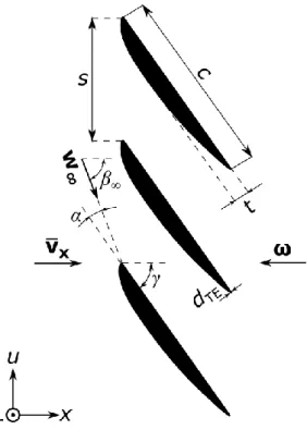
Such 3D effects are: centrifugal, and Coriolis force fields; near-endwall phenomena [26]; non-radial blade stacking, i.e. blade sweep and skew [27]; chordwise vortex filaments shed from the TE associated with spanwise changing blade circulation due to controlled vortex design [28]. According to the 2D assumption, the rotor is viewed as consisting of elemental annular blade cascades enclosed in the cylindrical stream tubes. This fluid mechanics view is consistent with the aeroacoustics approach in [29], suggesting that noise measurement data obtained for basic 2D, rectilinear models of blade sections can be adapted to rotating blades by means of spanwise segment splitting. As a great benefit of the 2D approach, an elemental annular cascade can be developed into a 2D cascade plane. The resultant 2D elemental blade cascade is illustrated in Figure 2. Furthermore, only 2D, cylindrical streamsurfaces have been covered by the present investigation, by neglecting of the radial velocity component in the preliminary design phase as suggested e.g. in [30].
12
In accordance with the 2D approach described above, the subjects of literature case studies focussing on systematic PVS experimentation are 2D, rectilinear profiles exposed to uniform, steady flow [1, 2, 7, 9-11, 13-19]. All of the aforementioned references are related to symmetrical profiles, i.e. either profiles out of the NACA00 series or flat plates. Some reports publish data, mostly via particular case studies, on PVS related to asymmetrical blade profiles [6, 9-10, 20, 31-33, 38], being more relevant to realistic axial fan design than symmetrical profiles.
The principal variables being potentially relevant to PVS have been gathered and grouped in Table 1 from two aspects: the rotor geometry based on the 2D elemental cascade (Figure 2) and the operational conditions.
Figure 2. 2D elemental blade cascade
13 Table 1. Quantities influencing PVS
Elemental 2D cascade geometry
Variable Symbol Dimension [SI]
chord length c m
TE thickness dTE m
roughness height k m
blade count N 1
radius r m
maximum thickness of blade profile
t m
stagger angle γ 1
Operational characteristics
Variable Symbol Dimension [SI]
angle of attack α 1
rotational speed n = ω/2π 1/s
free-stream turbulence intensity
TI 1
a) State variables of the fluid
absolute temperature T K
14
density ρ kg/m3
b) Material properties of the fluid
specific gas constant Rsp
J/(kg·K) ≡
m2/(s2·K)
heat capacity ratio κ 1
dynamic viscosity μ kg/(m·s)
c) User demand mean axial velocity through
the cascade, related to volume flow rate
vx m/s
total pressure rise Δpt Pa ≡ kg/(m·s2) d) Modelling result
PVS frequency f 1/s
Additional variables are introduced, corresponding to the turbomachinery analysis [24, 25] and having a potential influence on PVS. It is noted that these are not new independent variables but derived from the variables in Table 1. The derived variables are as follows:
The blade spacing:
s N r N
r, 2 (1)
15 The sound speed:
a RT R
T, sp, (2)
The free-stream velocity:
v w
vx x
, cos (3)
where is the flow angle.
Due to the rotational system, the effect of the centrifugal and the Coriolis force fields are to be considered:
cf 2
)2
2 (
,n r n r g
r (4)
sin Cor
) 2 ( sin ,
, n w n w g
w (5)
Considering the coordinate system illustrated in Figure 2, the vector of centrifugal force field intensity points radially outward, yielding a positive sign in Eq. 4. The vector of Coriolis force field intensity expressed as 2w∞ , points radially inward, corresponding to a negative sign in Eq. 5.
With the use of these purposefully introduced variables, the 18 independent quantities playing potentially a role in the PVS phenomenon are collected as follows.
TI, α, c, dTE, k, r, s, t, f, T, a, w∞, gc, gCor, μ, ρ, Δpt, Rsp
Since n is not listed among the above variables, gcf is truly independent, and therefore, ω can be expressed using r and gcf.With similar logic, gCor is also independent because β∞, appearing as a characteristic in Eq.
(5) in addition to the formerly discussed ones, is neither listed above. t and dTE were included in the table because they represent the extension of the blade profile in the chord-normal direction, and, as such, they are presumed to influence the VS phenomenon. It is noted that, according to [9-10, 33], the size of the
16
laminar separation bubble as well as its distance from the TE play a significant role in the PVS phenomenon.
However, these characteristics are presumed to be dependent on α, c, w∞, and μ, and, as such, they are already implicitly included in Table 1.
The above-listed independent characteristics are further processed herein in a comprehensive manner by means of dimensional analysis.
3) Execution of dimensional analysis
Based on [34-35], dimensional analysis as a mathematical method is applied to facilitate the determination of the dimensionless quantities playing a potential role in the PVS phenomenon in case of low-speed axial fan rotor blades. A brief and concise scope of the mathematical method of the dimensional analysis is presented in Appendix A.
Utilizing the feature of the dimensional analysis that the dimensionless quantities can be combined with each other, can be multiplied by a constant, or their arbitrary power can be taken, the dimensionless variables presented in Table 2 have been obtained.
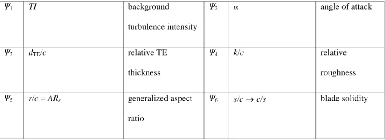
Table 2. Dimensionless quantities
Ψ1 TI background
turbulence intensity
Ψ2 α angle of attack
Ψ3 dTE/c relative TE
thickness
Ψ4 k/c relative
roughness Ψ5 r/c = ARr generalized aspect
ratio
Ψ6 s/c c/s blade solidity
17
Ψ7 t/c maximum relative
thickness
Ψ8
Stc
w c f
chord Strouhal number Ψ9
a M w w
a
Mach number Ψ10 2
cf cf
2 2
cf Fr
c g
w w
c
g
Froude number (centrifugal)
Ψ11 2
Cor Cor
2 2
Cor Fr
c g
w w
c
g
Froude number (Coriolis)
Ψ12
Rec
c w c
w
chord Reynolds
number Ψ13
T R
p Ψ
w p w
p
sp t 14 2
t 2
t 1
p p p p
p
t t
total pressure ratio Ψ14
2 dyn sp 2
sp
2 p
p w
T R w
T
R
p Eu
p
dyn
Euler number
4) Results and discussion
The dimensional analysis draws attention to the approximations relevant to PVS modelling. Simplifying assumptions, validity ranges, and boundary conditions can be systematically specified on the basis of the above-listed dimensionless quantities. The physical modelling related to PVS involves measurement case studies using the following conditions [1, 2, 7, 9-11, 13-19]:
i. steady, isolated blade profile,
ii. the blade profile is placed in a uniform, steady flow, iii. the TE is perpendicular to the flow direction.
In what follows, the obtained nondimensional quantities are systematically discussed from the perspective of reasonability and limits of PVS modelling approximations relevant to low-speed axial fans.
18
a) Free-stream turbulence intensity (Ψ1 = TI). Since the PVS phenomenon is related to the BL transition process, TI has a significant influence on its characteristics [9, 10, 39]. As the TI is increased, the transition in the attached and initially laminar BL may prevent the BL from separation, thus deactivating the feedback loop mechanism. Therefore, the TI is to be critically viewed and monitored in PVS experiments. In most cases, measurements on PVS were performed [2, 9, 11, 13-14, 18] in a wind tunnel in which the characteristic free-stream turbulence intensity did not exceed 0.1%. However, in [15], the TI is limited to 0.3%. Recently in [10], PVS was detected at turbulence intensities up to 0.8%, being in accordance with the present authors’ measurement campaign [38]. In [18], PVS measurements were carried out at TI of around 1%. These references suggest that TI ≤ 1% is a condition for which the PVS phenomenon probably occurs.
b) Relative roughness (Ψ3 = k/c). As will be demonstrated later, the coefficient CD plays a substantial role in the semi-empirical model for PVS frequency prediction [32, 37]. The effect of relative roughness is discussed herein via its influence on CD. In general, in a 2D flow approach, CD is the function of the following characteristics:
Re k c
C
CD D, c, (6)
The effect of roughness is discussed herein with an analogy to pipe friction. In determining the friction loss coefficient λ for pipes, the concept of hydraulic smoothness is as follows. A pipe is termed "hydraulically smooth" at a given Re if a reduction in the relative roughness does not cause a reduction in λ. Therefore, for hydraulically smooth pipes, λ is a function of Re only, and does not depend on the relative roughness.
In analogy to this concept, hydraulically smooth blade profiles are considered herein. This means that a reduction in k/c does not cause a reduction in CD. Therefore, the effect of k/c is neglected herein, and CD is determined as a function of α and Rec only, as the following equation illustrates. In the turbomachinery
19
literature, e.g. [24], measured CD data are often provided without any specification of k/c. For such cases, in lack of further information, hydraulic smoothness has been assumed here as simplifying assumption.
Rec
C
CD D , (7)
In addition to the blade geometrical data specified in Table 2, i.e. t/c and dTE/c, further details of the blade profile geometry (e.g. effect of the individual shape of the camber line) are considered to be implicitly taken into account via the drag coefficient, as discussed later.
c) Aspect ratio (Ψ5 = ARr). This quantity is related to the following characteristics: extension of the blade in radial direction, i.e. blade span; and distance of the elemental blade cascade under consideration from the endwalls (annulus walls). Ψ5 = r/c, termed herein as generalized aspect ratio, draws the attention that the AR of the blade, i.e. the blade span-to-chord ratio, plays a role in the PVS phenomenon. Generally, the PVS noise peaks become more and more dominant as the AR decreases, as reported in [1]. Most of the measurements [2, 9-10, 13-15] are related to an AR of 2.5 - 3.5; although in [11, 13] and [7], PVS was detected in case of an AR of 2 and 1.875, respectively. Only a few reports, e.g. elaborated by the research group of the present authors [37, 38], regard PVS studies on endwall-bounded blade models of finite AR, being relevant for realistic axial fan blades. The semi-empirical model available for prediction of PVS frequency in [32, 37] relies on the drag coefficient CD valid for a 2D, i.e. infinite AR, case. As the experiments in [36-38] suggest, the PVS frequency predicted in such 2D view is a fair approximation – within the uncertainty limits of the semi-empirical model – even for the PVS frequency detected at midspan of finite-AR blade models with the constraint of AR ≥ 1.5. The semi-empirical model will be discussed later.
d) Blade solidity (Ψ6 = c/s). Based on [24], if c/s ≤ 0.7, the aerodynamics of the blades in the cascade can be modelled in an isolated blade approach. Therefore, in a critical view, the results of PVS measurements on isolated blade profiles can be adopted only to such low-solidity rotor cases. For further generalization of the presented approach in rotor analysis, the following note is added. In the isolated blade approach,
20
upon need and agreement by the analyzer, the inlet relative flow angle β1 may be selected and consequently considered through the entire analysis instead of β∞.
e-f) Centrifugal and Coriolis force fields (Ψ10 = Frcf , Ψ11 = FrCor). The appearance of Frcf and FrCor in the list of dimensionless characteristics draws attention to the fact that the impact of centrifugal and Coriolis force fields on PVS is to be considered in a realistic fan rotor. The experiments on steady airfoils [1, 2, 7, 9-11, 13-19] are in lack of such force fields. Therefore, the systematic and comprehensive investigation of their effect on PVS in fan rotors is a subject of future research.
g) Reynolds number (Ψ12 = Rec). According to [9], PVS may occur only within a certain Reynolds number range, and this range depends on the angle of attack (α), and the relative thickness of the blade profile (t/c).
In the case of low-speed axial fan blades, the relative thickness is usually less than 10 to 15 %, which corresponds to a lower limit of Rec,low ≈ 50 000 [32, 37-38], as considered in what follows. The upper limit depends on the critical Reynolds number triggering the natural laminar-to-turbulent transition.
h) Mach number (Ψ9 = M). The energy equation between an arbitrary A point characterized by velocity w∞
and an also arbitrary T stagnation point on the rotor blade surface can be written in the co-rotating system approximately as follows, assuming an isentropic process:
T A p 2
2 T T
c
w (8)
By expressing the first term in Eq. (8) with the use of Mach number, Eq. (8) can be written as follows:
T 2
A 2
1 M 1 T
T
(9)
The density change is limited herein to 2 %, i.e. (ρT / ρA) ≤ 1.02, with the following consequences. i) As a reasonable engineering approximation, this yields that the density is considered to be constant, and is characterized by the density at the suction port of the fan (ρ ≈ constant ≡ ρS). ii) The isentropic
21
approximation results in a temperature change of (TT / TA) ≤ 1.01. On this basis, the temperature change is neglected, and the temperature is approximated by the absolute temperature at the suction port of the fan (T ≈ constant ≡ TS). In reality, the process is not truly isentropic but polytrophic, due to heat transfer.
Therefore, the temperature tends to be equalized, leading to temperature changes even less than 1 %. From the above, the limiting Mach number for low-speed fans is obtained as follows by assuming isentropic process (Appendix B):
2 . 1 0
1
2 T A 1
M (10)
Therefore, the limit of M ≤ 0.2, being relevant to low-speed fans, yields that the PVS process can be investigated with the simplifying assumptions of ρ ≈ constant ≡ ρS, and T ≈ constant ≡ TS.
i) Euler number (Ψ14 = Eu). Utilizing the former M ≤ 0.2 criterion, and neglecting the density change through the rotor, the Euler number can be written as follows (Appendix C):
03 . 2 0
dyn M2
p
p
(11)
As a result of Eq. (11), the dynamic pressure on the suction side can be neglected in comparison to the static pressure, thus the following inlet condition can be obtained: pS,T ≈ pS = ρSRspTS. Therefore, Eu manifests a dimensionless inlet pressure boundary condition to the flow through the elemental cascade, as a ratio between the characteristic dynamic pressure and the inlet pressure of pS,T ≈ pS = ρSRspTS. Due to this approximation, the Ψ14 can be written as follows:
S,T P,T
S,T S,T t
S S t t
p p p
p p p
p p p
p
p
(12)
22
j) Total pressure ratio (Ψ13 = (Δpt + pS,T)/pS,T ). On the basis of Eq. (12), and assuming an isentropic process, the following limitation can be obtained for the total pressure ratio. Here, the relative change of density has been approximated by the upper limit of 2 % as stated below Eq. (9).
03 . 1 02 . 1
>
>
S P
S P
T S,
T P, stat
t
p p p p p
p (13)
A total pressure ratio limitation of pP,T / pS,T ≤ 1.03 is in accordance with the former reasoning. For instance, a pS = 105 Pa value corresponds to Δpt = 3000 Pa, covering the practical range of low-speed axial flow fans.
The discussion related to Eqs. (8) to (13) is in accordance with the standard [40] stating that a distinction between the stagnation and static values of temperature, pressure, and density shall be made only if M >
0.2. It is to be noted that, although the M ≤0.2 limitation enables the assumption of constant density and temperature in the case of measurements on steady airfoils [1, 2, 7, 9-11, 13-19], such experiments cannot represent the enthalpy-increasing process manifested in the total pressure ratio of pP,T / pS,T > 1 relevant to fans. In fact, pP,T / pS,T is below unity in a steady airfoil-study, due to the inevitable losses. As a contrast, the PVS phenomenon occurs in a flow field exposed to enthalpy increase in a realistic fan. Such an effect is to be systematically investigated in future studies.
An intermediate summary of the discussion made so far is given as follows, providing rules of thumb on PVS modelling, based on the literature as well as on the experiences by the present authors.
a) The results of physical modelling of PVS involving measurements on isolated, steady models of blade profiles [1, 2, 7, 9-11, 13-19] can be adopted to blades of realistic low-speed axial fan rotors if the following conditions are fulfilled for both the physical modelling and the real rotor case.
TI ≤ 1%
k/c 0, i.e. hydraulic smoothness
23 AR ≥ 1.5
c/s ≤ 0.7 Rec ≥ 50 000
M ≤ 0.2, i.e. Eu ≤ 0.03
If any of these necessary conditions is violated, additional studies are necessary for confirming the occurrence of PVS as well as for investigating the transferability of the results of physical modelling to real rotors. Such studies may involve e.g.: grids generating inlet turbulence for obtaining higher TI (e.g. to be adopted to fans with inlet protection grille); cascade experiments for c/s > 0.7 (e.g. to extend the validity of modelling beyond propeller-type fans); studies on roughened blades for obtaining higher k/c (e. g. to model the effect of blade surface roughening due to abrasion during fan operation).
b) Even if the above necessary conditions are fulfilled, the PVS experiments on steady models of blades are in lack of modelling the phenomena related to centrifugal and Coriolis force fields, as well as enthalpy increase. This yields arbitrary modelling constraints of Frcf = 0, FrCor = 0, and pP,T / pS,T < 1.
Since the aforementioned phenomena are substantial in realistic fan rotors, their impact on PVS will be investigated in the future by the present authors by systematically changing the Frcf, FrCor, and pP,T / pS,T characteristics in comparative case studies.
c) Out of the initial pool of the 14 dimensionless quantities listed in Table 2, the following ones have remained yet undiscussed: α, dTE/c, t/c, and Stc.
Ψ2 = α Ψ3 = dTE/c Ψ7 = t/c Ψ8 = Stc
24
In what follows, their relationship will be discussed via the semi-empirical modelling approach outlined in [32, 37].
5) Semi-empirical model for predicting the PVS frequency
In further discussing the group of [α, dTE/c, t/c, Stc], it is purposeful at this point to introduce b, i.e. the transversal distance between the shed vortex rows, as an alternative length scaling parameter for the Strouhal number. This means that b, as an additional independent characteristic, is added to the pool of quantities listed in Table 1, without processing it in the dimensional analysis. Stc is multiplied by the dimensionless ratio of b/c, thus resulting in the following definition of “universal” Strouhal number:
18 .
* 0
w
b
St f (14)
As demonstrated in Eq. (14), and emphasized already in the Introduction, the benefit of such Strouhal number is that, according to the measurement experiences [14-15, 32], it can be regarded as constant.
Therefore, it provides a straightforward means for predicting the PVS frequency f. Recently, the present authors have extended the “universality” of the St* 0,18 constant to asymmetric blade profiles relevant to low-speed axial fans, such as the circular arc-cambered plate of 8 % relative camber, and the RAF-6E airfoil [38]. For these profiles, the average value of the universal Strouhal number, taking into account the measurement uncertainty, was found to be St* = 0.19±0.03. This range fits well to the average value suggested in the literature (Eq. 14). The uncertainty of the universal Strouhal number draws the attention to the following modelling approximation: the ambition of any PVS frequency estimation attempt may be limited to the determination of the 1/3 octave band. The results in [10], showing a variation in the PVS frequency, are in accordance with this view.
25
In what follows, efforts are to be made for empirical determination of b/c as a function of the further dimensionless quantities listed above.
As outlined in the Introduction, the PVS phenomenon is strongly related to the characteristics of the BL.
Therefore, a correlation is presumed to exist between b and a thickness-type property of the BL at the TE, i.e. in the near wake. For involving the BL thickness in the discussion, the pool of nondimensional quantities is supplemented with the blade drag coefficient CD, being a widely used empirical characteristics in turbomachinery analysis and preliminary design. The role of CD was already indicated in the “Relative roughness” subsection. As detailed in [21, 32, 37, 41], the following relationship is valid between CD and Θ, the momentum thickness of the blade wake. Using this relationship, the wake thickness is implicitly included in the empirical modelling of b/c with the use of CD.
c
CD2Θ (15)
A semi-empirical model has been elaborated in [32] for determining b/c. This model is under further development [37]. This semi-empirical model synthesizes the PVS data obtained for isolated steady blade models, as well as other case studies [1-2, 14-17, 31]. Without going into details but referring to [32] for further information, the empirical model expresses the following relationship. The dependence of the drag coefficient on further parameters has been discussed in the “Relative roughness” subsection.
d c t c C Rec
c b c
b , T E , , D , (16)
By means of this relationship, the entire pool of nondimensional quantities set in Table 2, supplemented purposefully with b/c and CD, has been covered with the discussion on PVS.
26 6) Special notes on the semi-empirical model
a) Obtainment of f and b from the measurement data. The PVS measurements carried out on further blade models are to be evaluated in the future for confirming the universality of St* as well as for extending the experimental database of the semi-empirical model. For such purposes, it is necessary to determine f and b from the measurement data. f can be obtained e.g. from the spectral analysis of acoustics or hot-wire measurements. The specialties in obtaining b are commented on in what follows.
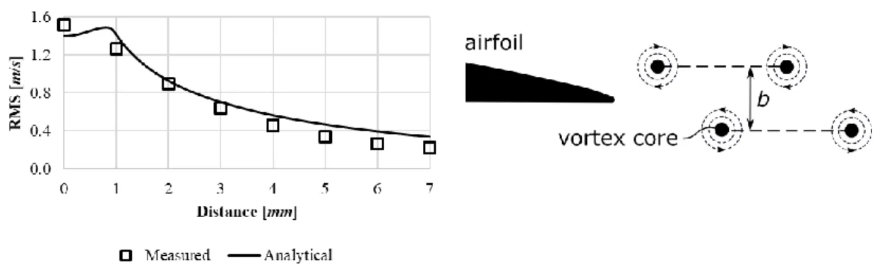
According to [14, 15], b has been considered as the transversal distance between the two maxima of the root-mean-square (RMS) of the velocity fluctuation measured by means of multicomponent hot-wire anemometry. The present authors concluded that the application of a single-component hot-wire is a reasonable compromise for determining b [38]. As a support to this conclusion, the authors developed an analytical model on the vortex-generated velocity fluctuation RMS, on the basis of the Rankine vortex approach, for comparison to the single-hot-wire-measured RMS distribution [38]. The illustrative example in Figure 3 shows that the analytical RMS distribution can be fit well to the measured one. By means of best-fitting, the centre of the shed vortex row can be localized. Accomplishing such a fitting process for both shed vortex rows, b can be determined as the transversal distance between the vortex centres.
Regarding Fig. 3, it is noted that the analytical distribution, based on the Rankine model, exhibits an unrealistic local RMS peak near the vortex centre, at the radius of the vortex core. The involvement of advanced vortex models, such as the Scully (Kaufmann) model [42, 43], may offer a potential perspective for smoothing this phantom peak, providing a better fit of the analytical RMS distributions to the measurement data. Such model development is in progress.
27
Figure 3. Fluctuating velocity RMS distributions (the x-axis denotes the transversal distance from vortex center), and illustration of the shedding vortices
b) Reynolds number effect. As formerly outlined, CD, utilized in the semi-empirical model, exhibits a Reynolds number-dependence. Such dependence is to be considered in predicting f on the basis of St*. The literature is limited in reporting on force coefficients for moderate Reynolds numbers. For illustrative comparison, detailed lift and drag coefficient data have been reproduced by the present authors from the literature, for an airfoil profile – left column, NACA23012 profile [44] –, and for a cambered plate – right column, 417a profile [45]. The sketches of the two profiles are shown in Figure 4. Figure 5 shows the comparative lift and drag plots for the two profiles for Reynolds numbers in the order of magnitude of 104. Figure 6 presents the force coefficients for the cambered plate for an extended Reynolds number range.
Figure 4. The blade profiles taken as examples [44, 45]
28
Figure 5. Lift and drag coefficients at moderate Reynolds numbers. Left column: NACA23012 profile [44]. Right column: 417a cambered plate [45].
Figure 6. Lift and drag coefficients for the cambered plate [45]
The data in Figs. 5 to 6 draw attention to the following. a) Notable variation in the drag coefficient as a function of Reynolds number. This yields that the Reynolds number effect on the frequency of the PVS phenomenon, usually occurring for Rec ≥ 5104, manifests itself via the drag coefficient. b) Notable
29
Reynolds-number-dependence in the lift coefficient. Since the lift coefficient is related to the isentropic total pressure rise performed by the rotor cascade [24, 25], such dependence is to be considered in preliminary fan design. c) For moderate Reynolds numbers, the drag coefficient is substantially less for the cambered plate than for the airfoil. This emphasizes the potential for exploitation of cambered plates in low-speed fan design for the moderate Reynolds number range, in advance to airfoil profiles, in terms of better lift-to-drag ratio, and thus, better efficiency – but keeping in mind the PVS-related possible noise and vibration issues.
In order to estimate the order of magnitude of the effect of Re-dependence of CL and CD, the following illustrative example is given. Taking a realistic and representative low-speed axial flow fan [46] as a reference, Rec varies along the blade span within the range of 30000 - 200000, due to the variation in the chord and in the flow velocity (the latter is also influenced by the rotor speed, 700 to 1400 1/min). Based on Figure 6, this variability in the Reynolds number may cause a variation in CL and CD up to 20 % and 30
%, respectively, depending on the α angle of attack. The effect of such variance in CL is to be considered in preliminary fan design since it tends to influence the isentropic total pressure rise [24, 25]. On the other hand, CD is related to the distance between the shed vortex rows via the momentum thickness of blade wake (Eq. (15)). For this reason, due to the variation in the drag coefficient CD (Re), the PVS frequency may vary within a bandwidth of 30 % of the middle frequency in the presented example.
7) Summary and future remarks
Dimensional analysis has been applied as a comprehensive means for obtaining the dimensionless quantities playing a potential role in the PVS phenomenon. On this basis, the limitations and approximations related to the presently available experimental techniques on PVS have been discussed from the perspective of transferability of the literature data on PVS from steady, isolated blade profile models to low-speed axial fan rotors. The conclusions are formulated as follows.
30
a) The literature has critically been overviewed in a systematic and comprehensive manner, in terms of all dimensionless characteristics. Limitations and simplifying assumptions have been given for the dimensionless characteristics as necessary conditions for transferability of PVS measurement data on isolated, steady airfoils to realistic blades of axial fan rotors. The limitations and assumptions are summarized in Table 3.
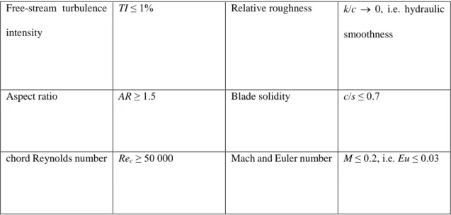
Table 3. Limitations and simplifying assumptions for PVS modelling Free-stream turbulence
intensity
TI ≤ 1% Relative roughness k/c 0, i.e. hydraulic smoothness
Aspect ratio AR ≥ 1.5 Blade solidity c/s ≤ 0.7
chord Reynolds number Rec ≥ 50 000 Mach and Euler number M ≤ 0.2, i.e. Eu ≤ 0.03
b) Further dimensionless characteristics have been considered via the semi-empirical modeling approach outlined in Section 5. These characteristics are collected in Table 4.
31 Table 4. Semi-empirical model parameters
Angle of attack α Relative TE thickness dTE/c
Maximum relative thickness
t/c Chord Strouhal number Stc
With introducing b, i. e. the transversal distance between the shed vortex rows, as an alternative length scaling parameter for the Strouhal number, the “universal” Strouhal number proposed by the literature has been derived, according to Eq. (14). As it has been emphasized, switching to the universal Strouhal number definition, i.e. St* 0,18, provides a straightforward method for estimating the PVS frequency. The modelling uncertainty of the semi-empirical model, incorporating the uncertainty of St*, yields that the ambition of PVS frequency prediction is restricted to the determination of the 1/3 octave band involving the PVS frequency.
The paper outlines some specialties related to the semi-empirical model. On the one hand, utilizing the analytical vortex model developed by the present authors, data obtained by a single-component hot-wire are suitable for determining b. Further development of the analytical model involving an advanced vortex model is a future research task for obtaining more reliable results on b. On the other hand, the effect of the Reynolds number on PVS has been represented through comparative measurement data reproduced from the literature. The notable Reynolds number dependence of both the lift and drag coefficients – with the latter having an influence on the PVS phenomenon – is illustrated for a moderate Reynolds number range, being typical for the PVS phenomenon.
32
c) The dimensional analysis pointed to topics uncovered in the open literature so far in investigating the PVS phenomenon. On this basis, the authors have formulated the following objectives of systematic future research on PVS related to low-speed axial fan rotor blades. Remarks have been given for the related research methodology.
i. 2D flow assumption. The available PVS data are obtained from measurements on 2D rectilinear profiles exposed to steady, uniform flow. It is to be critically analyzed how realistic 3D rotor flow effects influence the PVS phenomenon. Examples for such effects are as follows, being fully neglected in the experiments: centrifugal and Coriolis forces acting on the blade BLs; near-endwall effects such as annulus wall BLs, corner stall, and tip leakage flow; blade sweep and skew; swept and/or staggered blade trailing edge; 3D effects due to spanwise changing blade circulation. For the latter item, it is to be investigated how the nearly-chordwise vortex filaments shed from the blade due to controlled vortex design interact with the nearly-spanwise vortex filaments due to PVS.
ii. Neglect of streamwise increase in ambient pressure. The available PVS data are related to airfoils exposed to a free jet. It is to be critically investigated how the streamwise increase of pressure in the environment of the shed vortices, occurring in a realistic rotor blade passage, acts on the PVS process.
iii. Limited blade solidity. The available PVS data are related to isolated profiles, causing an applicability limit of ≤ 0,7 in terms of blade solidity. However, it is to be investigated how the increase of blade solidity influences the PVS phenomenon.
iv. Reynolds number. At moderate Reynolds number, in a rotating system, the circumferential velocity u, representing a solid body rotation, dominates in w∞, thus w∞ tends to increase with the blade radius. As a result, the chord Reynolds number increases as well. Therefore, it is to be investigated how the spanwise changing Reynolds number affects the PVS characteristics.
33
An effective means of further research is the extensive involvement of Computational Fluid Dynamics (CFD) in the PVS studies. A carefully designed CFD campaign can effectively treat the various effects in a well-distinguished manner. For example, a periodic rotor blade passage is sufficient to be modelled, and centrifugal as well as Coriolis forces can either be taken into account [47] or neglected for judging the significance of the effect of such force fields on the PVS phenomenon. Purposefully selected basic experiments are to be carried out for validating the CFD tools. The overall effect of PVS is eventually to be evaluated on spectral noise and vibration measurements on real axial fan rotors.
Funding
This work has been supported by the Hungarian National Research, Development and Innovation (NRDI) Centre under contract No. NKFI K 129023. The research reported in this paper and carried out at BME has been supported by the NRDI Fund (TKP2020 IES, Grant No. BME-IE-WAT and TKP2020 NC, Grant No.
BME-NCS) based on the charter of bolster issued by the NRDI Office under the auspices of the Ministry for Innovation and Technology. The contribution of Gábor DAKU has been supported by Gedeon Richter Talent Foundation (registered office: 1103 Budapest, Gyömrői út 19-21.), established by Gedeon Richter Plc., within the framework of the “Gedeon Richter PhD Scholarship.”
Declaration of Conflicting Interests
The author(s) declared no potential conflicts of interest with respect to the research, authorship, and/or publication of this article.
Appendix
Appendix A. Method of dimensional analysis
Any correlation between physical variables Q1, Q2, … QNv of number Nv can be expressed as follows:
0 ) ,...
, (
F1 Q1 Q2 QNv (A.1)
34
where F1 is an a priori unknown function. According to reference [34], the above equation is reducible to the following form:
0 ) ,...
, (
F2 Ψ1Ψ2 ΨNp (A.2)
where F2 is also an a priori unknown function, Np the number of the dimensionless quantities, and Ψ1, Ψ2,
…, ΨNp are the dimensionless quantities, obtained as products of the powers of Q1, Q2, …, QNv. The relation between Nv and Np can be written as follows:
DM v
p N R
N (A.3)
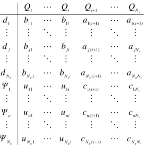
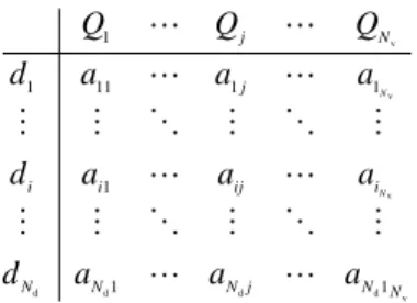
where RDM is the rank of the Dimensional Matrix (DM). The dimensions of each variable are given by the DM, in which the rows are the principal (SI) dimensions d1, d2, …, dNd (e.g. meter, second, kilogram etc.), where Nd indicate the number of principal dimensions, and the columns are the variables Q1, Q2, …, QNv
(e.g. velocity, density, dynamic viscosity etc.). Any aij element of this matrix is the exponent to which the particular dimension is raised in the particular variable (Figure 3).
d v d
d d
v v v
1 1
1
1 1
11 1
1
N N j
N N
N
i ij
i i
j
N j
a a
a d
a a
a d
a a
a d
Q Q
Q
N N
Figure A.1. The Dimensional Matrix (DM)
The DM is composed of submatrices A and B in the following way. The A matrix is the rightmost largest quadratic submatrix, which has RDM rows and columns. The B matrix is assembled by the residual elements, so it has RDM rows and (Nv - RDM) columns. A technique is presented in [35] by means of which the
35
dimensionless variables can be quickly and conveniently determined from the Dimensional Set (DS) (Figure A.2).
Figure A.2. The Dimensional Set (DS) [35]
The DS is formed by four matrices A, B, C, and U (as shown in Figure A.3), where C can be calculated in accordance with the aforementioned technique as follows:
T 1 ) (A B
C (A.4)
which has (Nv - Nd) rows and Nd columns. The U matrix is the unit matrix, which has (Nv - Nd) rows and columns, and any uij element is defined as follows:
j i
j uij i
if 0
if
1 (A.5)
36
v p p
p p
p
v v v d d
d d
d
v v
) 1 ( 1
) 1 ( 1
1 )
1 ( 1 1 11
1
) 1 ( 1
) 1 ( 1
) 1 ( 1 )
1 ( 1 1 11
1
1 1
N N i
N i N N
N
nN i
n ni n
n
N i
i
N N i
N i N N
N
jN i
j ji j
j
i i
i
N i
i
c c
u Ψ u
c c
u Ψ u
c c
u Ψ u
a a
b b
d
a a
b b
d
a a
b b
d
Q Q
Q Q
Figure A.3. Example for DS
Thus, the dimensionless variables can be determined from the DS as follows:
p
1 1
, ...
, 2 , 1 where
v
N j
Q Ψ Q
i
k N
i k
c k u k n
jk
jk
(A.6.)
After the principal variables are determined, the next task is to give the appropriate sequence of the variables in the DM. In the following, an overview of some rules and guidelines is given for sequencing the physical variables in the DS based on [35]:
a) If there is a dimensionless physical variable in the DM, then this variable must be in the B matrix. In case of PVS, it means that the turbulence intensity (TI), and angle of attack (α) must be in matrix B.
b) The A matrix must not include two or more variables with the same dimensions. Therefore, the A matrix may contain only one variable of the following: c, dTE, k, r, s, t.
c) It is generally advantageous to gather the dependent variables in matrix B because each one appears as exactly one dimensionless variable. By such means, we can guarantee the separation of the dependent variables from each other. Accordingly, the DM of PVS can be written as follows (Figure A.4):
37
0 0 1 0 1 0 0 0 0 0 0 0 0 0 0 0 0 0
0 1 0 0 2 2 1 2 2 1 1 0 0 0 0 0 0 0
3 1 0 1 2 1 1 1 1 1 0 1 1 1 1 1 0 0
1 0 0 0 0 1 1 0 0 0 0 0 0 0 0 0 0 0
sp t Cor
cf T E
K s m kg
w T c R p g
g a f t s r k d TI
Figure A.4. The DM of PVS The DS (upper left: B, upper right: A, left down: U, lower right: C):
0 2 1 0 1 0 0 0 0 0 0 0 0 0 0 0 0 0
1 2 0 0 0 1 0 0 0 0 0 0 0 0 0 0 0 0
1 1 0 1 0 0 1 0 0 0 0 0 0 0 0 0 0 0
0 2 0 1 0 0 0 1 0 0 0 0 0 0 0 0 0 0
0 2 0 1 0 0 0 0 1 0 0 0 0 0 0 0 0 0
0 1 0 0 0 0 0 0 0 1 0 0 0 0 0 0 0 0
0 1 0 1 0 0 0 0 0 0 1 0 0 0 0 0 0 0
0 0 0 1 0 0 0 0 0 0 0 1 0 0 0 0 0 0
0 0 0 1 0 0 0 0 0 0 0 0 1 0 0 0 0 0
0 0 0 1 0 0 0 0 0 0 0 0 0 1 0 0 0 0
0 0 0 1 0 0 0 0 0 0 0 0 0 0 1 0 0 0
0 0 0 1 0 0 0 0 0 0 0 0 0 0 0 1 0 0
0 0 0 0 0 0 0 0 0 0 0 0 0 0 0 0 1 0
0 0 0 0 0 0 0 0 0 0 0 0 0 0 0 0 0 1
1 0 1 0 1 0 0 0 0 0 0 0 0 0 0 0 0 0
0 0 0 0 2 2 1 2 2 1 1 0 0 0 0 0 0 0
3 1 0 1 2 1 1 1 1 1 0 1 1 1 1 1 0 0
1 1 0 0 0 1 1 0 0 0 0 0 0 0 0 0 0 0
14 13 12 11 10 9 8 7 6 5 4 3 2 1
sp t Cor
cf T E
Ψ Ψ Ψ Ψ Ψ Ψ Ψ Ψ Ψ Ψ Ψ Ψ Ψ Ψ K
s m kg
w T c R p g
g a f t s r k d
TI
Figure A.5. The DS of PVS

![Figure 5. Lift and drag coefficients at moderate Reynolds numbers. Left column: NACA23012 profile [44]](https://thumb-eu.123doks.com/thumbv2/9dokorg/743608.30776/28.892.138.765.209.586/figure-lift-coefficients-moderate-reynolds-numbers-column-profile.webp)
![Figure A.2. The Dimensional Set (DS) [35]](https://thumb-eu.123doks.com/thumbv2/9dokorg/743608.30776/35.892.247.657.291.591/figure-a-the-dimensional-set-ds.webp)