A New Sliding Mode Speed Observer of Electric Motor Drive Based on Fuzzy-Logic
Chiheb Ben Regaya, Abderrahmen Zaafouri, Abdelkader Chaari
Unit C3S, High School of Sciences and Techniques of Tunis (ESSTT), 5 Av. Taha Hussein, BP 56, 1008 Tunis, Tunisia
E-mails: chiheb.benregaya@enseignant.edunet.tn;
abderrahmen.zaafouri@isetr.rnu.tn; assil.chaari@esstt.rnu.tn
Abstract: In this paper, the speed of the induction machine is controlled by a variable structure controller. To eliminate speed sensor we use a sliding mode observer based on fuzzy logic “FSMSO”. The control algorithm and observation is emphasized by simulation tests and it is comapred with the classical sliding mode speed observer”SMSO”. Analysis of the results shows the characteristic robustness to disturbances of the load and the speed variation for the FSMSO than SMSO.
Keywords: induction motor; fuzzy sliding mode speed observer; sliding mode control;
sliding mode speed observer; vector control
1 Introduction
Vector control is the most common technique used to control the induction motor, since it offers performance very close to that of the dc motor. But it remains sensitive to parametric variation. For this reason a lot of research has proposed nonlinear control laws with parameter identification and state estimation [1-4].
Among them, the back stepping control, the sliding mode control. The latter has a good performance and is insensitive to parametric variations [5, 6].
But the use of sign functions in control law or observer allows the appearance of the chettering phenomenon that can exite the high frequencies qnd the latter can damage the system [7, 8]. To alleviate this drawback, several solutions have been proposed, such as using a transition band around the sliding surface, or an integrator block in the controller output [9, 10]. In both solutions the phenomenon of chattering is surely reduced, but the tracking error remains.
To make the observer more robust to to disturbances of the load and the speed variation while reducing the chattering phenomenon, we propose in our paper a
sliding mode speed control with a new sliding mode speed observer based on fuzzy logic.
In this paper, in addition to the sliding mode speed control, a speed observation system based on fuzzy logic comprising a current observer, a rotor flux observer and a rotor speed observer, is presented for an indirect vector control of an induction motor drive. The present paper is organized as follows: in Section 2, the model of induction motor is defined. The sliding mode control of speed is established in Section 3. In Section 4, the classical sliding mode speed observer is developed. The fuzzy sliding mode speed observer is the subject of the fifth part.
We close our paper with a conclusion.
2 Induction Motor Modeling
In a reference connected to the stator, we can express the model of the induction machine by the following state equation [1, 3]:
11 12 1
21 22 0
s s
s
r r
s
i A A i B
d v
A A
dt
i Cx
(1)
Where:
T
s s s
i i i :Stator current;
T
s s s
v v v :Stator voltage;
T
r r r
:Rotor flux;
Rs,Rr : Resistance of Stator and Rotor;
Ls,Lr : Stator and Rotor inductance;
M : Mutual inductance;
2
1 M L Ls r
: Total leakage factor;
r Lr Rr
: Rotor time constant;
r : Angular rotor speed;
11 1 s s 1 r
A R L I
112 s r r r
A M L L I J
21 r
A M I;A22rJ
1r
I
1 1 s
B L I;C
I 0
1 0 I 0 1
;
0 1
1 0
J
3 Sliding Mode Speed Control
The sliding mode control is a strategy to reduce the state trajectory to the sliding surface and to move it to the balance point [5].
The design of this type of control requires an appropriate choice of the switching surface, the state of convergence and the calculation of the control law.
The model of the induction machine can be represented by the following mechanical equation:
3 2
r em r r
em dr qs qr ds
r
j d C C f
dt
C pM i i
L
(2) For representation in the state space, we set:
* 1
2 1
r r
x
x d x
dt
(3)
The speed error is processed by a variable structure controller for generating the control signal U. To cancel the static and reduce the effect of chattering, we add an integrator to the sliding mode regulator with a response time τ. The simplified model can be written as follows:
1 1
2 2
0 1 0
0 1
x x
f U
x x
j j
(4)
To have a response to the system fast without overshoot, the right commutation or sliding surface can be chosen as follows:
x 1 1
S x x
(5)
With υ the slope of sliding line.
The control law is defined as follows:
1 1 2 1
U x x
(6) Where ψ1and ψ2 are coefficient of the sliding mode to be designed.
With:
1 1 2 1
1 2
1 1 2 1
0 0
0 0
x x
x x
if S x if S x
if S x if S x
(7)
The convergence condition is defined by the Lyapunov equation in order to make the area attractive and invariant [5, 9].
x x x
1
1
1
1 0S S S f j j x j x
(8) Condition (8) is true if:
x
1
1 0 and x
1
1 0S f j j x S j x
(9)
From equation (9) we can write the expression of α1,2 and β1,2 as follows:
1 1
1 2
1 1
1 2
0 0
0
0 0
0
x x x x
S x
f S x f j j
S x
if S x f j j
(10)
Then
1 1
2 2
0 f j j
(11)
4 Sliding Mode Speed Observer
It is an observer of flux and current based on the sliding mode method. This observer has the advantage of not requiring input speed and rotor time constant unlike other observers. Thus, any variation of these quantities will not affect the estimation of current and flux [6, 9].
In addition, the use of sliding mode technical methods for the design of the observer ensures on the one hand the robustness with respect to various disturbances, and on the ohter the good dynamic performance.
The system of equation (1) can be described as follows:
11 11 1
11
s r s s s
r r s
d i A i A i v
dt
d A i
dt
(12)
Where:
11 11 11 11 11
1 1 ,
, 1 ,
r r
s r r
r
r s
M L L
A M A A A I A
S matrix is defined by:
11
1
1
r
r s
r
r s
r r s
r r
M i
S A i
i
(13)
We note that the matrix S appears simultaneously in the equations of flux and currents. This implies that the design of the observer for current and flux can be based on the replacement of the common term, which is the matrix S by the same sliding function ϑ:
1 2
1 ˆ ˆ ˆ
ˆ ˆ
ˆ ˆ
ˆ 1
r
r s
r
r s
r r r
M i
S i
(14)
The observers of currents and flux can be written as follows:
11 1
ˆ ˆ ˆ
ˆ ˆ
s s s
r
di A i v
dt d dt
(15) Where:
1 0
2 0
u sign S u sign S
(16)
ˆ ˆ ˆ
ˆ ˆ ˆ ,
ˆ , ˆ
T T
s s s r r r
s s s s s s
i i i
S i i i S i i i
With
1 0
1 0
1 0
1 0
sign S if S
if S sign S if S
if S
ˆs,ˆs and s, s
i i i i are respectively the components observed and measured stator current. Flux estimation is a simple integration of sliding mode functions when the estimated current converges to the measured current without the need to know the speed or the rotor time constant. The selection of u0 will guarantee the convergence of the current observation by Lyapunov stability analysis.
It is worth noting that we have supposed that the equivalent control of sliding mode observer is achieved by a simple low-pass filtering the discontinuous control [9].
1,2 1,2
1 1
eq
s
(17) μ is the time constant of the low pass filter.
Now the rotor flux can be estimated by the following equation:
1 2
ˆ ˆ
eq r
eq r
(18)
The angle of the rotor flux can be calculated as follows:
ˆ tan 1 ˆr ˆr
(19)
Using equation (14), we can calculate the estimate rotor speed as follows:
1 2
1 ˆ ˆ ˆ ˆ
ˆ ˆ
eq eq
r r s r Bs
r r
r
M M
i i
(20)
The block diagram of the sliding mode observer of the currents, flux and speed is given in the figure below:
Current observer
Sliding mode functions
ˆs
i
ˆs
i
Flux observer
1
2 ds,qs
i i
ds, qs
v v ˆr
Equation (15) Equation (16) Equation (18) ˆr
ˆr
Speed estimator
Equation (20)
Figure 1
Schematic diagram of sliding mode observer
The stability of the observer can be proved by the Lyapunov stability theory. The Lyapunov function is chosen as follows [6]:
1 2
T n n
L I I
(21)
Where
n s s
I i i
The Lyapunov function V is positive definite, which satisfies the Lyapunov stability. The derivative of L is:
T n n
LI I
(22)
To satisfy the Lyapunov stability, the second condition must satisfyL0. From Equation (12) and (15), we have:
11n r
I A I
(23)
Equations (22) become:
11 0T T
LI r A I I
(24) Note that: u sign I0 ( )
We can find the expression of constant u0:
11 0
T T
r
s s
I A I I
u
i i
(25)
With:
2 2
11 11
T r r
r s r r s r r
r r
T
s s
I i i
A I I A i i
5 Fuzzy-Sliding Mode Speed Observer
In this section, fuzzy logic and sliding mode are combined together to give us a new concept of observer. The observer thus obtained is called fuzzy sliding mode speed observer. It presents the same structure as the SMSO given in Section 4, but the sliding function ϑ will be replaced by a fuzzy controller. So after the calculation of the sliding function ϑ, we can use the Equation 15 to estimate the currents and rotor flux in oder to estimate the rotor speed using the following equation:
1 2
1 ˆ ˆ ˆ ˆ
ˆr ˆ r r s r r Bs
r
M M
i i
(26)
The idea of this combination is inspired by the fact that in the ideal case when S(α, β) is far from the sliding surface, ϑ must have a very large value and when S(α, β) is near the sliding surface ϑ must have a small value.
The block diagram of the fuzzy logic calculation of ϑ used in our simulation is given in the figure below:
S
1
2 Sk k
Figure 2
Block diagram of the adaptation mechanism of the sliding function ϑ using fuzzy logic When choosing the linguistic value, it should be taken into account that the control must be robust and time of calculation adopted by the fuzzy controller should not be high to not slow down the process [11-13]. In this proposed linguistic method we have used 5 rules.
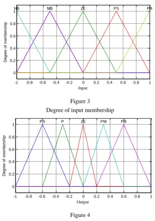
For fuzzyfication, we have chosen triangular fuzzyfication and for deffuzzyfication the centroid deffuzzyfication method is used in the proposed method.
All fuzzy variables have the same universe of discourse (Sα, Sβ, Δϑ)and are divided into five fuzzy sets (NB, NS, ZE, PS, PB) for the input variables and (PS, P, ZE, PM, PB). Membership functions are chosen in the form triangular as in Figures 3 and 4.
Figure 3 Degree of input membership
Figure 4
Degree of output membership
In terms of numerical values, the behavior of this mechanism is characterized by action law shown in Figure 5. Indeed, for each input values the mechanism generates a variation of Δϑ which corresponds to the increase or decrease of sliding function ϑ.
Rule 1: If S(α,β) is NB So Δϑ is PB.
Rule 2: If S(α,β) is NS So Δϑ is PM.
Rule 3: If S(α,β) is ZE So Δϑ is ZE.
Rule 4: If S(α,β) is PS So Δϑ is P.
Rule 5: If S(α,β) is PB So Δϑ is PS.
-1 -0.8 -0.6 -0.4 -0.2 0 0.2 0.4 0.6 0.8 1
0 0.2 0.4 0.6 0.8 1
Input
Degree of membership
NS ZE PS
NB NS PB
-1 -0.8 -0.6 -0.4 -0.2 0 0.2 0.4 0.6 0.8 1
0 0.2 0.4 0.6 0.8 1
Output
Degree of membership
PS P ZE PM PB
Figure 5
Variation law of fuzzy controller for sliding function ϑ adaptation
5 Simulation Results and Discussion
To assess the proposed algorithm, the solution has been checked using Matlab – Simulink in order to validate the fuzzy sliding mode speed observer for estimating the rotor speed. The parameters of the three phase induction motor are given in Table 1.
Table 1
Parameters of induction motor
Designation Notations Rating values
Stator resistance Rs 2.3
Rotor resistance Rr 1.83
Stator self-inductance Ls 261 mH Rotor self-inductance Lr 261 mH
Mutual inductance M 245 mH
Moment of inertia j 0.03 kgm2 Friction coefficient f 0.002 Nm
Number of poles p 2
Rated voltage Vsn 220 V
Figure 6 shows the architecture of the vector control algorithm incorporating the fuzzy sliding mode speed observer.
-1 -0.8 -0.6 -0.4 -0.2 0 0.2 0.4 0.6 0.8 1
-0.8 -0.6 -0.4 -0.2 0 0.2 0.4 0.6
Input
Output
E
ˆg
ˆr IM3~
Reference flux Sliding mode Speed control
Currents control
dq abc
Slip estimator
dq
abc
αβ abc αβ
abc
Mech. Load Tload
Sensors
Vabc*
Iabc
*
Vds
*
Vqs
*
iqs
*
ids
ids
iqs
dq
I
V
Fuzzy sliding mode speed observer
Figure 6
Block diagram of the vector control including speed fuzzy sliding mode observer
Figures 7 and 8 show the test of tracking speed for the machine by considering the nominal conditions. These figures represent the dynamic responses of the electromagnetic torque and the speed. The performance is checked in terms of load torque and speed variations. Very good tracking speed is obtained.
Figure 7
Torque response for step varying of load torque (FSMSO and SMSO)
0 0.5 1 1.5 2 2.5 3
-60 -40 -20 0 20 40 60
Electromagnetic T orque
T ime [s]
Cr , Te
Reference FSMSO SMSO
2.5 2.55 2.6 2.65 2.7
8 9 10 11 12
Zoom
Figure 8
Estimated speed using FSMSO and SMSO
Figures 7 and 8 show the simulation results to a step speed (314rd/s) under a load torque of 10 Nm. The estimated speed by the sliding mode speed observer and the fuzzy sliding mode speed observer are nearly similar (Figure 8). We can see the effect of the chattering phenomenon on the speed estimated reponse, this is due to the nature of the sliding functions. Figure 7 shows the electromagnetic torque and the effect of chattering phenomenon developed during the starting and the stationary phase.
Figure 9
Speed estimation error for the SMSO and FSMSO
Figure 9 shows the speed estimation error for both types of observers. It is clear that the estimation error for FSMSO is smaller than the error for SMSO which is caused by the sliding mode functions.
0 0.5 1 1.5 2 2.5 3
-300 -200 -100 0 100 200 300 400
Rot or speed
T ime [s]
ref , r
Reference FSMSO SMSO
2.5 2.55 2.6
-314.4 -314.2 -314 -313.8
SMSO
FSMSO
e e
Zoom
Results obtained show clearly the superiority of FSMSO compared to SMSO for the speed estimation and minimization of the ripple effect (chattering phenomenon).
Conclusions
A sliding mode control and speed estimation algorithm based on current and flux observers are proposed in this paper. In this algorithm fuzzy sliding mode functions are selected to control and determine rotor speed that is assumed to be unknown. The proposed scheme validated by simulation results shows the superiority of FSMSO compared to SMSO for the speed estimation and reducing of the chattering phenomenon. This algorithm can be improved further by using an adaptive approach for the rotor and stator resistance variations, and will be implemented in the future work on a digital processor (DSP) to validate the proposed scheme.
References
[1] Ben Regaya, C., Farhani, F., Zaafouri, A., Chaari, A. "Comparison between Two Methods for Adjusting the Rotor Resistance", International Review on Modelling & Simulations (I.RE.MO.S.) 2012, Vol. 5, N. 2, pp. 938-944 [2] Derdiyok, A. "A Novel Speed Estimation Algorithm for Induction
Machines", Electric Power Systems Research, 2003, Vol. 64, N. 1, pp. 73- 80
[3] Farhani, F., Ben Regaya, C., Zaafouri, A., Chaari, A. "On-Line Efficiency Optimization of Induction Machine Drive with Both Rotor and Stator Resistances Estimation", International Review on Modelling & Simulations (I.RE.MO.S.) 2012, Vol. 5, N. 2, pp. 930-9937
[4] Cheng-Hung, T. "CMAC-based Speed Estimation Method for Sensorless Vector Control of Induction Motor Drive", Electric Power Components and Systems, 2006, Vol 34, N. 11, pp. 1213-1230
[5] Zhao, Junhui, Caisheng Wang, Feng Lin, Le Yi Wang, and Zhong Chen.
"Novel Integration Sliding Mode Speed Controller for Vector Controlled Induction Machines", IEEE Power and Energy Society General Meeting, 2011, pp. 1-6
[6] G. R. Arab Markadeh. "A Current-based Output Feedback Mode Control for Speed Sensorless Induction Machine Drive using Adaptive Sliding Mode Flux Observer", The Fifth International Conference on Power Electronics and Drive Systems, 2003, PEDS 2003, Vol. 1, pp. 226-231 [7] Karim Khémiri. "Novel Optimal Recursive Filter for State and Fault
Estimation of Linear Stochastic Systems with Unknown Disturbances", International Journal of Applied Mathematics and Computer Science, 2011, Vol. 21, N. 4, pp. 629-637
[8] Tichy, Michael. "On Algebraic Aggregation Methods in Additive Preconditioning", Department of Mathematics, University of Würzburg, 2011
[9] Mezouar, A. "Adaptive Sliding-Mode-Observer for Sensorless Induction Motor Drive using Two-Time-Scale Approach", Simulation Modelling Practice and Theory, 2008, Vol. 16, N. 9, pp. 1323-1336
[10] Rehman, H., Gilven, M. K., Derdiyok, A., Longya Xu. "A New Current Model Flux Observer Insensitive to Rotor Time Constant and Rotor Speed for DFO Control of Induction Machine", Power Electronics Specialists Conference. PESC. 2001 IEEE 32nd Annual, 2001, Vol. 2, pp. 1179-1184 [11] Kouzi, K., Nait-Said, M. S., Hilairet, M., Bertholt, E. "A Robust Fuzzy
Speed Estimation for Vector Control of an Induction Motor", 6th International Multi-Conference on Systems Signals and Devices, 2009, SSD `09, pp. 1-6
[12] Khan, Md. Haseeb. "Fuzzy Logic-based HPWM-MRAS Speed Observer for Sensorless Control of Induction Motor Drive", Journal of Engineering
& Applied Sciences, 2010, Vol. 5, N. 4, pp. 86-93
[13] wei-Ling Chiang. "Adaptive Fuzzy Sliding Mode Control for Base-isolated Buildings" International Journal on Artificial Intelligence Tools, 2000, Vol. 9, N. 4, pp. 493-503