Sliding Mode Control of a Wind Turbine with Exponential Reaching Law
Abderrahmen Mechter, Karim Kemih, Malek Ghanes*
L2EI Laboratory, Jijel University, BP 98, Oued Aissa, Jijel, Algeria
* ECS-Lab ENSEA, Cergy-Pontoise, 95014, France
a.mechter@ensea.fr, karim.kemih@ensea.fr, ghanes@ensea.fr
Abstract: This paper presents a novel control strategy of a wind turbine based on Doubly Fed Induction Generator (DFIG) to maximize the electrical power generated by the DFIG, for low wind speed. To achieve this objective, the nonlinear sliding mode control with exponential reaching law (ERL ), the Bees algorithm and the fuzzy maximum power point tracking MPPT are applied to the system. The ERL and the Bees algorithm are used to obtain a good reference tracking and to suppress the chatter phenomenon. The effectiveness of this control strategy is proven through the simulation results.
Keywords: Wind Energy; Doubly fed induction generator; Sliding Mode Control;
Exponential Reaching Law; Bees algorithm; fuzzy maximum power point tracking
1 Introduction
Wind energy conversion is the fastest-growing energy source among the new power generation sources in the world. Advances in wind turbine technology made necessary the design of more powerful control systems. This is in order to improve wind turbines behavior, namely to make them more profitable and more reliable.
Many control strategies have been studied and applied to optimize the power for low wind speed: in reference [2] a fuzzy logic and a second order sliding mode controller were presented, the control scheme based on feedback linearization and gain scheduled linear quadratic regulator (LQR) is applied for the control of a wind turbine in [3]. In reference [4] a nonlinear state feedback PI controller with an estimator was used to optimize the power; a comparative study on the performance between PI and SMC controllers is presented in [5]. Reference [6]
has developed an adaptive feedback linearization controller; a fuzzy-PI controller is used to extract an optimal power from the wind turbine system based on the Permanent Magnet Synchronous Generator in [7]. In reference [8] an RST controller is used to optimize the produced power, an LQG controller based on the
R
G
mecC
tP
tP
elinearized wind turbine model was used in [9]. In reference [10], a variable structure control based on a sliding mode control has been presented, and a robust nonlinear controller has been presented in [11].
The objective of this paper is the control of active and reactive powers in the variable speed wind turbine. For this, we must continually adjust the turbine rotational speed according to the wind speed. The nonlinear sliding mode control with an exponential reaching law is used to achieve our objective. In [12], [13]
and [14], the authors have used the conventional sliding-mode control to control the power produced by a wind turbine, but in this paper, we will use the same method but by employing an exponential reaching law (ERL) proposed by Fallaha et al. [15] to calculate the control law, the fuzzy maximum power point tracking MPPT to determine the rotational speed reference and the Bees algorithm to determine the optimal parameters of the controller. The advantage of the proposed approach is that allows to obtain a good reference tracking and the suppression of chatter phenomenon.
This paper is organized as follows. Firstly, In Section 2, the wind turbine configuration is presented. In Section 3, the sliding mode control is used to establish the control law applied to the system. Finally, the simulation results are given to show the efficacy of the proposed approach.
2 Wind Turbine Systems
A wind turbine generally consistes of a wind rotor, drive shaft, gear system and a generator, as presented in Fig. 1 [16]. The wind turbine consists of several blades (mostly three blades). The wind turbine rotates at a speed which depends on the wind speed. This speed will be adapted to that of the electric generator through a gearbox.
Figure 1
One-mass wind turbine model
The energy recovered by the wind turbine rotor is given by:
1 2 3
t p 2
P C ρπR v
(1) Where, is the air density [Kg / m3], R is the blade length [m ], v represents the wind speed [m / s]. Cpis the power coefficient; it depends on the tip speed ratio
λ and the pitch angle of the blades
. It is given by [17]:
31 0 035 21
0 08 1
3
1 0 035
0 5109 116 0 4 5
0 08 1
0 0068
. λ . β β p
C λ, β . . . β e
λ . β β
. λ
(2)
The tip-speed ratio
λ is defined as:RΩt
λ v (3)
Ωt, is the mechanical angular speed of the turbine [rad / sec].
The mechanical torque and the mechanical angular speed are given by:
0 5 2 3
1 1 t 1 p
mec t
t t
mec t
. C ρπR v
C C P
G G Ω G Ω
Ω GΩ
(4)
Ctis the mechanical torque [N.m] and G is the multiplication ratio.
The mechanical angular speed is determined by applying the fundamental equation of dynamic:
mec mec em mec
JΩ C C fΩ (5) Where:
Jis the total inertia of the rotating parts [Kg.m2], f is the coefficient of viscous damping, and Cem is the electromagnetic torque of the generator [N.m].
The electrical and magnetic equations of the DFIG are given by:
s ABC s s ABC s ABC
r ABC r r ABC r ABC
V R I d φ
dt
V R I d φ
dt
. (6)
s ABC ss s ABC sr r ABC
t
r ABC rr r ABC sr s ABC
φ L I M I
φ L I M I
(7)
Where,
s s s
ss s s s
s s s
l m m
L m l m
m m l
,
rr rr rr rrr r r
l m m
L m l m
m m l
,
1 3 2
2 1 3
3 2 1
sr
m m m
M m m m
m m m
and
1
2
3
2 3 2
3
sr
sr
sr
m m cos θ m m cos θ π . m m cos θ π
Where:
Vsis the stator voltage.
Vris the rotor voltage.
φsis the stator flux.
φris the rotor flux.
Rsis the stator resistance.
Rris the rotor resistance.
lsis the inductance of stator phase.
lris the inductance of rotor phase.
msis the mutual inductance between two stator phases.
mris the mutual inductance between two rotor phases.
msris the maximum of the mutual inductance between the stator and the rotor.
In the three-phase plan, the representation of asynchronous machine is difficult because it is strongly coupled. So it is necessary to represent the machine behavior in a two-phase plane given by the transformation of Park (Fig. 2).
a) DFIG representation on a three-phase plane b) DFIG representation on a two-phase plane Figure 2
The Park Transformation
The Park reference frame is given by the following set of equations [18-19]:
sd s sd sd s sq
sq s sq sq s sd
rd r rd rd sl rq
rq r rq rq sl rd
V R I d φ ω φ
dt
V R I d φ ω φ
dt
V R I d φ ω φ
dt
V R I d φ ω φ
dt
(8)
Where, ωsl ωsPΩmec.
sd s sd m rd
sq s sq m rq
rd r rd m sd
rq r rq m sq
φ L I L I
φ L I L I
φ L I L I
φ L I L I
(9)
Where,
sd sq
V , V , direct and quadrature voltages on the stator axis.
rd rq
V , V , direct and quadrature voltages on the rotor axis.
sd sq
I , I , direct and quadrature stator currents.
rd rq
I , I , direct and quadrature rotor currents.
ωs, the stator currents pulsation.
P, the number of machine poles pairs.
sd sq
φ , φ , direct and quadrature stator flux.
rd rq
φ , φ , direct and quadrature rotor flux.
Ls, the stator inductance.
Lr, the rotor inductance.
Lm, the mutual inductance between the stator and the rotor.
The stator active and reactive powers of the DFIG are given by [20],
3 2 3 2
s sd sd sq sq
s sq sd sd sq
P V I V I
Q V I V I
(10)
3 Control Strategy
As it is shown in Fig. 1, there are two control parts (mechanical and electrical parts). For each one, we will design a sliding mode controller. The optimal rotational speed of the turbine corresponds to opt and 0. It is used as a reference for the controller to determine the command (electromagnetic torque) that will be applied to the generator. The difficulty in controlling the DFIG is due to the coupling between the stator and rotor.
To simplify the task, the model is approximated to that of a DC machine. By orienting d axis in the direction of the flux s. We obtain:
0
sd s
sq
(11) Taking into account of (9), we obtain:
0
m sq
sd rd
sd s sd m rd s s s
sq s sq m rq m
sq rq
s
L V
I I
L I L I L L
L I L I L
I I
L
(12)
The rotor flux can be written as:
m sq
rd r rd
s s
rq r rq
L I L V L L I
(13)
If we neglect the stator resistance (for medium and high-power machines), and we make the stator flux constant (ensured by a stable grid connected to the stator).
We obtain the direct and quadrature voltages on the stator axis:
sd 0
sq s sd
V
V
(14) Taking into account (10) and (12), we obtain the stator active and reactive powers:
2
3 2 3 3
2 2
m
s sq rq
s m sq
s sq rd
s s s
P L V I
L L V
Q V I
L L
(15)
Taking into account equations (8) and (13), we obtain the direct and quadrature voltages on the rotor axis:
2 2
2 2
m m
rd r rd r rd sl r rq
s s
m m
rq r rq r rq sl r rd
s s
m sq sl
s s
L L
V R I L I L I
L L
L L
V R I L I L I
L L
L V L
(16)
The optimal stator active and reactive powers given by (17) are used as reference for controllers to calculate commands (Vrdand Vrq) that will be applied to the DFIG rotor.
5 3
2 3
0
opt p
s t
opt s
P C R
Q ( To ensure unity power factor )
(17)
The synthesis of these commands (Vrd. and Vrq. ) is represented thereafter, using the nonlinear sliding mode control with exponential reaching law.
4 Sliding Mode Control
The sliding mode control belongs to the family of a variable structure controllers.
The advantage of this method is its simplicity and robustness in spite of uncertainties in the system and external disturbances.
It consists of designing a control law that helps, to attract the state vector toward the sliding surface and to slide on the surface until reaching the equilibrium point (Fig. 3) [21-23].
We consider a nonlinear system defined as:
( n )
x ( t )f ( x,t ) b( x,t )u( x,t ) (18) where, xis the state vector and f ( x,t ), b( x,t )are nonlinear functions and u is the control input.
Figure 3
Sliding mode in a phase plane (se e )
To design a sliding mode control law, we must firstly, choose the switching surface. We take the general form proposed by Slotine [24]:
n 1
S d e
dt
(19) Where, e x xd is the tracking error; xd is the desired state, n is the system order and is a positive coefficient.
After choosing the sliding surface, we must choose the control law where the reaching condition defined by Lyapunov equation satisfied,
0 SS t The control law has the following form,
eq disc
uu u (20)
e
0 s
Switching surface
Equilibrium point
e
In order that the condition (19) is verified at any time, S is chosen as follows [15]
(a complete study of sliding-mode with ERL can be found in [15]):
0 1 0
Sp
k S
S sat
e
(21) Where, k is the discontinuous gain,
00 1
0 1
rd / p
S ( )
t k k
is the desired
reaching time, 0 , 001 and p0 sat S
is the saturation function,
1 1
1 1
1 1
if S
S S S
sat if
if S
(22)
The use of saturation function instead of sign function is justified to avoid chattering phenomenon.
4.1 Wind Turbine Rotational Speed Command
In this part, we develop a law command to control the rotational speed. Taking into account of (8) and (10), we obtain,
5
2 2
1 2 3
3 3
0 5 p 1
mec mec mec em mec mec em
. R C
f C c c c C
J JG J
(23)
with
5
2 3 3 3
1
0 5. R Cp 1
f , c , c
c J
JG J
The tracking error is defined by, e mec dmec According to (18), the switching surface is given by,
d
mec mec
S e (24)
2 1
1 2 3
0 1 0
p
d d
mec mec mec mec em mec
S
k S
S c c c C sat
e
1 2 2 1
3 3 3
3 0 0
1
1
p
d
em mec mec mec
S
c c k S
C sat
c c c
c e
(25)
Where,
1 2 2
3 3 3
1
3 0 0
1
1
p
d
eq mec mec mec
disc S
c c
u c c c
k S
u sat
c e
(26)
4.2 Stator Active Power Command
In this part, we develop a law command to control the stator active power.
According to the first equation of (16), the quadrature currents on the rotor axis is given by:
4 5 6
2 2
r 1
rd rd sl rq rd rd rq rd
m m
r r
s s
I R I I V c I c I c V
L L
L L
L L
(27)
with: 4 5
2 6 2
r 1
sl
m m
r r
s s
c R , c
L L
L L
L
c
L
,
The tracking error is defined by, IrdIrdd
According to (18), the switching surface is given by,
d
rd rd
S e I I (28)
2
4 5 6
3 0 1 0
p
d d
rd rd rd rq rd rd
S
k S
S I I c I c I c V I sat
c e
5
4 2
6 6 6
6 3 0 0
1
1
p
d
rd rd rd rq
S
c
c k S
V I I I sat
c c c
c c e
(29)
Where,
4 5
6 6 6
2
6 3 0 0
1
1
p
d
eq rd rd rq
disc S
c c
u I I I
c c c
k S
u sat
c c e
(30)
4.3 Stator Reactive Power Command
In this section, we calculate the law command to control the stator reactive power.
According to the second equation of (16), the quadrature currents on the rotor axis is giver by:
2 2 2
1
sl m sq r
rq rq sl rd rq
m s r s m m
r r
s s
R L V
I I I V
L L L L L
L L
L L
7 8 9 10
rq rq rd rq
I c I c I c c V (31) with :
8 10
2 2 2
7 9
1
sl m sq r
sl
m s r s m m
r r
s s rq
R L V
, c , c
L L L L
c L L
c
L L L
,
The tracking error is defined by, IrqIrqd
According to (18), the switching surface is given by,
d
rq rq
S e I I . (32)
7 8 9 10
3
3 0 1 0
p
d d
rq rq rq rd rq rq
S
S I I c I c I c c V I
k S
sat
c e
7 8 9 3
10 10 10 10
10 3 0 0
1
1
p
d
rq rq rq rd
S
c c c k S
V I I I sat
c c c c
c c e
(33)
Where,
7 8 9
10 10 10 10
3
10 3 0 0
1
1
p
d
eq rq rq rd
disc S
c c c
u I I I
c c c c
k S
u sat
c c e
(34)
5 Simulation Results
The control strategy was applied to a 660-kW wind turbine using Matlab/Simulink software. The simulation results show the effectiveness of the control strategy used in this study. The parameters of the wind turbine are:
21 165 1 225 3 0 01
2
s
r s r m
R . m, G 39, J 28 Kg.m ,2 . Kg / m , R 0.0146 Ω, f .
0.0238 0.0306 0.0303
. R Ω, L H , L H , L 0.0299 H , P
Nominal frequency: 50Hz.
The exponential reaching law parameters: 0 0 08. ,p2, 1000,k3.
The optimal active power can be written with neglected losses as [11]:
d opt
s t
P P
Form (1) and (3) we have: Ps k 3mecwith
5 3 3
2G
max p
opt
C R
k
So,
5 3 3
2
3 2G
max
d s p
rq mec
sq m opt
C R
I L
V L
With mec is the estimated rotational speed and dmecis determined using the fuzzy maximum power point tracking MPPT proposed by S. Abdeddaim et al.
[25] to maximize the output power and to adjust in real time the rotational speed of wind turbines.
on the other hand, the optimal reactive power is set to zero to ensure a unity power factor operation of the studied wind turbine: Qsref 0 [25],
Or, form (15), we have : rdd sq
m s
I V
L
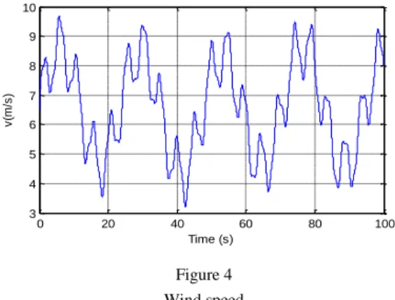
The Bees algorithm is employed to determine the control parameters k1, k2 and k3, it is an optimization algorithm inspired by the natural foraging behaviour of honey bees to find the optimal solution [26]. The parameters of the Bees algorithm are: the number of scout bees is 30, the number of best selected patche is 20, the number of elite selected patches is 10, the number of recruited bees around best selected patches is 15 and the number of recruited bees around elite selected patches is 30. In the literature, we can find many objective functions as a performance criterion. In this paper, we use the integral of time multiplied by squared error (ITSE), defined by :
2 0 tss
ITSE
te ( t ) Where tss is the final time.Fig. (4) present a variable wind profile comprised between 5 m/s and 12 m/s, and it varies under the nominal value (12 m/s). This allows observing the operation of the wind turbine for low wind speed.
0 20 40 60 80 100
3 4 5 6 7 8 9 10
Time (s)
v(m/s)
Figure 4 Wind speed
Fig. 5 shows the generator rotational speed under the proposed control method and the reference. We can see clearly that the estimated mec track perfectly the reference.
0 20 40 60 80 100
60 80 100 120 140 160 180
Time (s)
mec (rad/s)
mec
ref mec
Figure 5 Generator rotational speed
0 20 40 60 80 100
0 1 2 3 4
x 105
Time (s)
Ps (W)
Ps
ref Ps
Figure 6
Active power
The active and the reactive powers are presented in Fig. 6 and Fig. 7. As we can see, the powers converge to their desired references with good dynamics.
0 20 40 60 80 100
-2000 0 2000 4000 6000 8000 10000
Time (s)
Q s (VAR)
Qsref Qs
Figure 7
Reactive power
0 10 20 30 40 50 60 70 80 90 100
60 80 100 120 140 160 180
Time (s)
mecref &mec (rad/s)
mecref mecreaching law mecsat function
Figure 8
Generator rotational speed: comparaison between conventional sliding-mode control and sliding mode control with ERL and Bees algorithm
0 10 20 30 40 50 60 70 80 90 100
-0.5 0 0.5 1 1.5 2 2.5 3 3.5
x 105
Time (s) Psref & Ps (W)
Ps
ref P
s
sat function P
s reaching law
Figure 9
Active power: comparaison between conventional sliding-mode control and sliding mode control with ERL and Bees algorithm
0 10 20 30 40 50 60 70 80 90 100 -1000
0 1000 2000 3000 4000 5000 6000 7000 8000 9000
Time (s) Qsref & Qs (VAR)
Qs
ref Q
s
sat f unction Q
s reaching law
Figure 10
Reactive power: comparaison between conventional sliding-mode control and sliding mode control with ERL and Bees algorithm
Fig. 8, Fig. 9 and Fig. 10 represent a comparison between the conventional sliding-mode control and the sliding mode control with ERL and Bees algorithm.
These results show the effectiveness of the proposed approach, especially the very good tracking performance of the desired trajectory.
Conclusion
In this paper, the control of a 600-kW wind turbine for low wind speed was presented. To achieve this objective, the nonlinear sliding mode control with exponential reaching law and Bees algorithm are used to conceive the controllers of mechanical and electrical parts. The fuzzy maximum power point tracking MPPT is using to determine the rotational speed reference. The advantage of the proposed approach, compared to the conventional method is the good reference tracking and the suppression of chatter phenomenon. Simulation results show the effectiveness of the applied control strategy.
Acknowledgement
This work was supported by the CMEP- TASSILI project under Grant 14MDU920.
References
[1] T. Burton, D. Sharpe, N. Jenkins, E. Bossanyi: Wind Energy Handbook, John Wiley & Sons, Chichester, 2001
[2] S. Abdeddaim, A. Betka: Optimal Tracking and Robust Power Control of the DFIG Wind Turbine. International Journal of Electrical Power and Energy Systems, Vol. 49, 2013, pp. 234-242
[3] R. Burkart, K. Margellos, J. Lygeros: Nonlinear Control of Wind Turbines:
An Approach Based on Switched Linear Systems and Feedback Linearization. IEEE CDC-ECE, Orlando, 2011, pp. 5485-5490
[4] B. Boukhezzar, H. Siguerdidjane: Nonlinear Control with Wind Estimation of a DFIG Variable Speed Wind Turbine for Power Capture Optimization.
Energy Conversion and Management, Vol. 50, 2009, pp. 885-892
[5] D. Kairous, R. Wamkeue, B. Belmadani: Advanced Control of Variable Speed Wind Energy Conversion System with DFIG. IEEE EEEIC, Prague, 2010, pp. 41-44
[6] A. Mullane, G. Lightbody, R .Yacamini: Adaptive Control of Variable Speed Wind Turbines. Rev. Energ. Ren.: Power Engineering, 2001, pp.101- 110
[7] AG. Aissaoui et al. :A Fuzzy-PI Control to Extract an Optimal Power from Wind Turbine. Energy Conversion and Management, Vol. 65, 2013, pp.
688-696
[8] F. Hachicha, L. Krichen: Rotor Power Control in Doubly Fed Induction Generator Wind Turbine under Grid Faults. Energy, Vol. 44, 2012, pp. 853- 861
[9] B. Boukhezzar, H. Siguerdidjane: Comparison between Linear and Nonlinear Control Strategies for Variable Speed Wind Turbine Power Capture Optimization. Control Engineering Practice, Vol. 18, 2010, pp.
1357-1368
[10] Y. Bekakra, D. Ben attous: Active and Reactive Power Control of a DFIG with MPPT for Variable Speed Wind Energy Conversion using Sliding Mode Control. World Academy of Science, Engineering and Technology, Vol. 60, 2011, pp. 12-21
[11] K. Elkhatib, A. Aitouche, R. Ghorbani, M. Bayart: Robust Nonlinear Control of Wind Energy Conversion Systems. International Journal of Electrical Power and Energy Systems, Vol. 44, 2013, pp. 202-209
[12] Boubekeur, Boukezzar. Mohamed, M’Saad. : Robust Sliding Mode Control of a DFIG Variable Speed Wind Turbine for Power Production Optimization, Mediterranean Conference on Control and Automation, Ajaccio, 2008, pp. 795-800
[13] Kairous, D. Wamkeue, R. Belmadani, B.: Sliding Mode Control of DFIG based Variable Speed WECS with Flywheel Energy Storage, International Conference on Electrical Machines (ICEM), Rome, 2010, pp. 1-6
[14] Djilali, Kairous. René, Wamkeue. : Sliding-Mode Control Approach for Direct Power Control of WECS based DFIG, International Conference on Environment and Electrical Engineering (EEEIC), Rome, 2011, pp. 1-4 (2011)
[15] C. J. Fallaha et al. :Sliding Mode Robot Control With Exponential Reaching Law. IEEE Transactions on Industrial Electronics, Vol. 58, 2011, pp. 600-610
[16] N. Abu-Tabak : Stabilité dynamique des systèmes électriques multimachines: modélisation, commande, observation et simulation. PhD thesis. École centrale de Lyon, 2008
[17] S. Le-peng, T. De-dong, W. Debiao, L. Hui: Simulation for Strategy of Maximal Wind Energy Capture of Doubly Fed Induction Generators. IEEE ICCI, Beijing, 2010, pp. 869-873
[18] Hansen O. L: Aerodynamics of Wind Turbines. ISBN 978-1-84407-438-9.
Earthscan, London, Sterling VA, 2008
[19] F. K. A. Lima, E. H. Watanabe, P. Rodriguez, A. A. Luna: Simplified Model for Wind Turbine Based on Doubly Fed Induction Generator. IEEE ICEMS, Beijing, 2011, pp. 1-6
[20] S. T. Jou, S. B. Lee, Y. B. Park, K. B. Lee: Direct Power Control of a DFIG in Wind Turbines to Improve Dynamic Responses. Journal of Power Electronics, Vol. 9, 2009, pp. 781-790
[21] S. Y. Guo and L. Chen : Terminal Sliding Mode Control for Coordinated Motion of a Space Rigid Manipulator with External Disturbance, Applied Mathematics and Mechanics, Vol. 29, 2008, pp. 583-590
[22] K Széll and Korondi P: Mathematical Basis of Sliding Mode Control of an Uninterruptible Power Supply, Acta Polytechnica Hungarica Vol. 11, 2014, pp. 87-106
[23] C. Ben Regaya, A. Zaafouri, A. Chaari : A New Sliding Mode Speed Observer of Electric Motor Drive Based on Fuzzy-Logic, Acta Polytechnica Hungarica Vol. 11, 2014, pp. 219-232
[24] J. J. E. Slotine, W. LI: Applied Nonlinear Control. Prentice Hall Englewood Cliffs, ISBN 0-13-040890-5, New Jersey, 1991
[25] S. Abdeddaim and A. Betka: Optimal Tracking and Robust Power Control of the DFIG Wind Turbine, International Journal of Electrical Power and Energy Systems, Vol. 49, 2013, pp. 234–242
[26] L. Ozbakir, A. Baykasoglu, P. Tapkan: Bees Algorithm for Generalized Assignment Problem, Applied Mathematics and Computation, Vol. 215, 2010, pp. 3782-3795