hjic.mk.uni-pannon.hu DOI: 10.33927/hjic-2020-23
FOLLOW-UP CONTROL OF A SECOND ORDER SYSTEM IN SLIDING MODE
MÁRKDOMONKOS*1 ANDNÁNDORFINK1
1Department of Mechatronics, Optics and Mechanical Engineering Informatics, Budapest University of Technology and Economics, Bertalan Lajos u. 4-6, Budapest, 1111, HUNGARY
This paper deals with an instantaneous feedback controlled inverter using sliding mode control. The theoretical contribu- tion of this paper is that a common state-space-based sliding surface design method is extended for follow-up control.
Starting from the basic theory of sliding mode control, the trajectory of the error signal is modelled. The practical contri- bution of this paper is the relationship between the trajectory of the error signal and the Total Harmonic Distortion (THD) of the output voltage signal. The conditions of the sliding mode control using an Uninterruptible Power Supply (UPS) are discussed. A rectifier as a non-linear load is simulated. Experimentally validated simulation results are presented.
Keywords: sliding mode control, hysteresis control, second order system, UPS
1. Introduction
Power electronics equipment that produces alternating voltage and current impulses is typical of Variable Struc- ture Systems (VSSs). A VSS usually consists of a state when it is insensitive to variations in parameters and load disturbances. This state is referred to as the sliding mode.
The cost of insensitivity is an infinitely high switching frequency. Due to the limits with regard to switching de- lays and frequencies of controlled switches, an ideal slid- ing mode does not exist. However, the ideal sliding mode can be approximated with an acceptable degree of accu- racy.
The theory of Variable Structure Systems and slid- ing mode control was developed decades ago in the So- viet Union, mainly by Vadim I. Utkin [1] and David K.
Young [2]. According to the theory, sliding mode control should be robust but experiments have shown that it is subject to serious limitations. The main problem with ap- plying the sliding mode is the high frequency of oscilla- tion around the sliding surface, referred to as chattering, which strongly reduces the performance of the control.
Very few have managed to put the robust behavior pre- dicted by the theory into practice. Many have concluded that the presence of chattering makes the sliding mode control a good game theory, which is not applicable in practice. Over the following period, researchers invested most of their energy in chattering-free applications, lead- ing to the development of numerous solutions like the discrete-time sliding mode [3], sector sliding mode [4], adaptive sliding mode [5] and terminal sliding mode [6].
*Author for correspondence:domonkos@mogi.bme.hu
Sliding modes can also be used for feedback compensa- tion [7].
The design of a sliding mode controller consists of three main steps. The first is the design of the slid- ing surface, the second step is the design of the con- trol law which holds the system trajectory on the slid- ing surface, and the third and key step is implementation of the chattering-free sliding mode control. The system- atic sliding manifold design for linear systems was pro- posed by Utkin [1]. This method was extended in several ways and optimal sliding manifold designS proposed, e.g.
frequency-shaped sliding mode control (FSSMC) [8] sur- face design based onH∞control theory [9,10] and Ten- sor Product Model Transformation-based Sliding Surface Design [11]. The reference signal was constant in all the aforementioned papers. Recently, the application of pre- dictive control has become popular [12]. The new ele- ment in this paper is that the original method was ex- tended for Follow-up Control.
According to Refs. [13] and [14], Uninterruptible Power Supplies (UPSs) are being broadly adopted for the protection of sensitive loads, e.g. PCs, air traffic control systems, life care medical equipment, etc., against line failures or other perturbations in AC mains. Ideally, an UPS should be able to deliver: 1) a sinusoidal output volt- age with low total harmonic distortion during normal op- eration, even when feeding nonlinear loads (particularly rectified loads); 2) the voltage dip and recovery time due to a change in load step must be kept as small as possible, that is, provide a fast dynamic response; 3) the steady- state error between the sinusoidal reference and load reg- ulation must be zero. To achieve these, a Proportional In-
tegral (PI) controller is usually used [15], moreover, is- sues concerning robust stability and controller robustness are discussed in [16]. However, the system using the PI controller subject to a variable load rather than the nom- inal ones cannot produce a fast and stable output volt- age response. In the literature, some hybrid solutions to overcome this problem can be found [17,18]. The princi- ple of Pulse Width Modulation (PWM) plays a very im- portant role in power electronics [19]. In the field of in- verter technology, which produces a sinusoidal voltage, a great number of "optimized PWM" techniques have been proposed in the literature. These types of PWM invert- ers have very good steady-state characteristics, but for the voltage regulator to respond to a sudden change in the load takes a few cycles and nonlinear loads can cause high "load harmonics". This is unacceptable in UPS ap- plications for which instantaneous feedback is preferred [20,21]. The sliding mode control of power electronic inverters is suggested in Refs. [22] and [23]. On the one hand the main advantage of the sliding mode-based method proposed in this paper is the direct control of the transistor switches, but on the other hand uncontrolled THD results. That is why the THD is the focus of this paper.
The structure of this paper is as follows. After the In- troduction,Section 2presents the problem statement, de- scribes the system configuration and summarizes the de- sign of the sliding mode control.Section 3describes the equations of the system and shows how the mathematical foundations are applied to a practical example. Follow- ing the main steps of sliding mode design, namely the surface design, a control law is selected by taking into consideration the reduced chattering.Section 4presents the simulation results, which are validated by experimen- tal measurements of a10kVA UPS. Finally, inSection 5, the presented results are analyzed.
2. Problem Statement 2.1 System Configuration
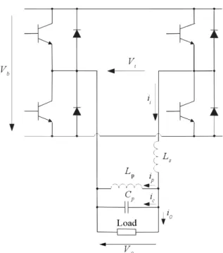
A simplified diagram of the inverter and filter is shown in Fig. 1Vbdenotes the battery voltage andvistands for the input voltage of the system, which is a filter with a load.
The input signal consists of three different values (Vb,
−Vband0) depending on the switching states of the tran- sistors. The goal is that the transistors must be switched in such a way thatvo, the output voltage of the system, follows the sinusoidal reference signal. Ls inFig.1 de- notes the leakage inductance of the transformer, which has a special structure to increase and set the value of Ls. The main field inductanceLpcannot be ignored from the point of view of the resonance circuit. The loss of the transformer is modelled by an increased load.
vo(t) =√
2·230 cos (2π50t) (1)
Figure 1:Simplified figure of the inverter and filter
2.2 Sliding Mode Control
A Single-Input Single-Output (SISO) system is given in state-space controllable canonical form.
˙
x(t) =Ax(t) +bu(t) (2)
y(t) =cx(t) (3)
wherex(t) ∈ Rn,A ∈ Rn×n,b ∈ Rn×1,c ∈ R1×n andu(t), y(t)∈R.y(t), the output variable of the con- trolled plant, can be described by an-th order differential equation supposing that the reference signalyr(t)can be differentiated at leastntimes.
The goal is given in
yr(t) =y(t)ift > Tc (4) whereTc denotes the control period. The system error, ey(t), is given by
ey(t) =yr(t)−y(t) (5) Thus the error signal,ey(t), can also be differentiated at least ntimes, so then−1-th derivative must exist and is continuous. Due to the latter property, when trying to eliminate the error, it is also useful to control its deriva- tives (including then−1-th derivative). Otherwise, be- cause of the system inertia, an oscillation with a large amplitude could arise. The essence of sliding mode con- trol could be summarized as follows: in order to elimi- nate the error in then-th dimensional phase space, a con- tinuous error trajectory running into the origin has been designed. Whilst planning, the physical limits should be taken into account. By implementing our very own tran- sient, the ideal system follows the reference signal with- out any errors. The control signal is designed so that the
trajectory realized does not deviate from the prescribed one or once the origin has been reached, it remains at rest.
Usuallyσ, a scalar variable, can be defined as a pos- itive or negative distance between the desired and actual trajectories, or each trajectory sector can be prescribed by a single scalar variable. The task of the controller is to ensure this scalar variable remains zero. In the classi- cal method of sliding mode control, this scalar variable is calculated as a linear combination of the error and its derivatives [1]. Whenn = 2, the scalar variable can be defined by the following equation:
σ(t) =ey(t) +τe˙y(t) (6) whereτ denotes a time constant-type control parameter chosen by us. In sliding mode control:
σ= 0 (7)
and the trajectory is described by the following equation:
ey(t) =−τe˙y(t) (8) that corresponds to a−1/τ gradient in the phase plane.
This is usually referred to as the sliding line or sliding surface in multidimensional phase space. The solution of Eq. 8is an exponential function with a negative exponent:
ey(t) =E0e−τt t≥0 (9) whereE0=ey(0). Consequently, the error will decrease according to the chosen time constant,τ, independently from the system parameters, e.g. load. After an exponen- tial transient process,yr(t) = y(t). To ensure that the system moves in all cases towards the sliding mode (i.e.
towardsσ(t) = 0), the following condition is necessary:
σ(t) ˙σ(t)≤0 (10) The design of a sliding mode controller does not re- quire accurate modelling, it is sufficient to only know the boundaries of the model parameters and the disturbance.
During sliding mode control, the only task is to switch the control signal so thatEq. 10is valid in every instance.
No other information concerning the controlled plant and the disturbances is needed. It is sufficient to determine whetherEq. 10holds or not. In simple cases (or within a range of errors and its derivatives), the signs of the control signal andσ(t)˙ are opposite. Thus it is often satisfactory to use a relay controller, which switches the control signal according to the sign of the parameterσ(t).
2.3 Follow-up Control
Sinceyr(t)is not constant,Wyr,u(s), the transfer func- tion fromu(t)(vi(t)) toyr(t)(vo(t)), must be calculated.
According toEq. 4, it is the inverse of the transfer func- tion with regard to the inverted system:
y(s) =Wu,y(s)u(s) (11)
Wyr,u(s) =Wu,y−1(s) (12) Usually, the inverse of Wu, y(s) cannot be realized. In our case,yr(t)is sinusoidal:
yr(t) =√
2Vrcos (ωrt) (13) Only two parameters must be calculated, namely the gain (Gr)and phase shift(ϕr)of the transfer function of the system at the reference angular frequency(ωr). The defi- nition of the error (Eq. 5) must be modified:
ey(t) =
√ 2 Gr
Vrcos (ωrt−ϕr)−y(t) (14)
3. Equations of the System
3.1 Filter and Load
Using the notation ofFig. 1, the equation for the currents is:
ii(t) =io(t) +ip(t) +ic(t) (15) By assuming resistive loadRL:
io(t) = 1 RL
vo(t) (16)
The equation of the input voltage is vi(t) =Ls
dii(t)
dt +vo(t) (17)
By substitutingEqs. 15and16intoEq. 17, the filter cir- cuit with a resistive load can be described by the follow- ing differential equation:
vi(t) =LsCp¨vo(t) + Ls RL
˙
vo(t) + 1
Gvo(t) (18) where
G= Lp
Ls+Lp
(19) The transfer function from u(t)(vi(t)) to yr(t)(vo(t)) (including the effect of the resistive load) can be calcu- lated from the Laplace transformed form ofEq. 18:
vo(s) = G
GLsCps2+GLRLss+ 1vi(s) =W(s)vi(s) (20)
3.2 The states of the state-space equation
Since the inverter and load are handled separately, the system has two inputs, namelyui andio. Since the in- put current must be calculated, three state variables are selected for the three storage elements, even if they are not independent and the rank of the system matrix is only 2. Using the notation ofFig. 1, the three state variables areii(t),ip(t)andvc(t):x(t) =
ii(t) ip(t) vo(t)
(21)
The load is connected in parallel to the inverter capacitor Cp. The load current includes the effect of transformer losses. The system has three outputs sincevo(t) = vc(t) as well as its derivative are necessary to calculate the scalar variable andii(t)is visualised. In the real system, the current of the capacitor is measured instead ofv˙o(t).
According toEqs. 15,16, and17, the matrices of the sys- tem are:
A=
0 0 −L1
s
0 0 L1
1 p
Cp −C1
p 0
B=
0 −L1
s
0 0
−C1
p 0
C =
1 0 0 0 1 0 0 0 1
D=
0 0 0 0 0 0
(22)
3.3 Error Trajectory
To calculate the error defined byEq. 14,Grandϕrmust first be calculated. According toEq. 20:
W(jωr) = G
GLsCp(jωr)2+GLRLsjωr+ 1 (23) Grandϕrcan be calculated fromEq. 23, whereW(jωr) denotes a simple complex number:
Gr=|W(jωr)| (24) ϕr=angle(W(jωr)) (25) Since the filter must be inductive,ϕr must be negative.
Therefore, the reference signal must lead tovo(t), which is the controlled signal inEq. 14:
y(t) =vo(t) (26) The derivative of the error is:
˙
ey(t) =−ωr
√2 Gr
Vrsin (ωrt−ϕr)−v˙o(t) (27) The scalar variable of the sliding mode control is calcu- lated byEq. 6.
3.4 Control Law
Three different control laws were examined. All of them can directly control the switching of the transistors. This is the main advantage of sliding mode control in the field of power electronics. More advanced controllers can be found inRef.[24].
Simple Relay
The input voltage on the filter is switched according to the sign ofσ(t):
vi(t) =Vbsign(σ(t)) (28) From a practical point of view, the main problems ofEq.
28are
• the inverter has a zero state, which is not applied;
• the switching frequency is uncontrolled.
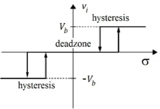
Figure 2:Double Relay with dead zone and hysteresis
Double Relay
The solution to the first problem is the usage of two re- lays:
vi(t) = Vb
2 sign(σ(t)) +Vb
2 sign(cos (ωrt−ϕr)) (29) Vband0are switched in the positive half period, while
−Vband0are switched in the negative half period. How- ever,Eq. 29does not solve the second problem.
Double Relay with dead zone and hysteresis
Both problems can be solved by a double relay with dead zone and hysteresis. This control law is shown inFig. 2.
3.5 Stability Analysis
Using a simple relay controller, whether or not Eq. 10 holds can be verified. First,σ(t)˙ must be expressed:
˙
σ(t) = ˙ey(t) +τ¨ey(t) (30) According toEq. 27:
¨
ey(t) =−ω2r
√2 Gr
Vrcos (ωrt−ϕr)−v¨o(t) (31)
¨
vo(t)can be expressed fromEq. 18:
¨
vo(t) = 1 LsCp
vi(t)− 1 RLCp
˙
vo(t)− 1 GLsCp
vo(t) (32) By substitutingEq. 28intoEq. 32:
¨
vo(t) = Vbsign(σ(t)) LsCp
− v˙o(t) RLCp
− vo(t) GLsCp
(33) According toEqs. 30and31, if the value of¨vo(t)is suffi- ciently large and the system operates in an area which is close enough to the sliding mode, then the sign ofv¨o(t) is the opposite to that of σ(t). From˙ Eq. 33, it is clear that if the value ofVbis sufficiently large and the system operates in an area which is close enough to the sliding mode, then the sign of¨vo(t)is the same as that ofσ(t). In conclusion, if the value ofVbis sufficiently large and the
system operates in an area which is close enough to the sliding mode, then the sign ofσ(t)is the opposite to that ofσ(t). Similar analyses can be conducted for all control˙ laws. In practice, the simulations proved that by substi- tuting the actual parameters of the system, all the control laws examined fulfil the condition (Eq. 10) during normal operations.
4. Simulation
MATLAB-Simulink simulations were carried out.
4.1 MATLAB-Simulink model
The main elements of the MATLAB-Simulink model are shown inFigs. 3–6. Even if the structure of the controller shown inFig. 6is quite simple, its performance is quite robust.
4.2 Model validation
The simulation results were compared to previous results measured by [25] as shown inFig. 7. The nominal power of the inverter is10VA. All parameters of (14) and (22) in addition to the values of dead zone and hysteresis shown inFig. 2are known fromRef.[25].
Like in real systems, where σis tuned manually to set the number of switches per period,σis changed to achieve a similar result in the simulation as in real sys- tems. The simulation result is shown inFig. 8 after the value ofσwas set.
The first problem faced in the simulation was the steady state. When the real system was measured, the screen of the oscilloscope seemed to be frozen for most settings ofσ. Therefore, the error trajectory was a closed curve during a period in a steady state.
Using the default settings of Simulink, a quasi-steady- state period of the error trajectory of the simulation re- sulted as is shown in Fig. 9. The consequent periods are slightly different, which causes subharmonics that are crucial from a practical point of view.
The main question is whether these subharmonics are an immanent property of the applied switching method or a result of an insufficiently precise simulation. Several simulations were carried out using different model con- figuration parameters in Simulink. It is concluded that the precise calculation of the switching instant is key to sim- ulating proper steady states. The Ode113(Adam) method is the most suitable integral method for switched systems.
(The equation solvers for UPS are compared inRef.[26]).
4.3 Analysis of the simulation results
The main advantage of the PWM technique is that the filter can be smaller resulting in a smaller no-load current.
The parameters of the filter are given in
Ls= 3.5mH,Lp= 32mH,Cp= 320µF (34)
Figure 3:The whole system.
Figure 4:Subsystem for calculating scalar variableS.
Figure 5:Subsystem for the load.
Figure 6:Subsystem for the relay controller of the dead zone and hysteresis
τ, the gradient of the switching line in the sliding mode, has been changed. The value of the nominal load is RL = 5.3Ω. The relationship between the gradient of the switching line and the number of switches is shown inFig. 10. The larger the value ofτ, the smaller the gra- dient of the switching line and the greater the number of switches per period. On the other hand, the bigger the value of τ, the longer the transient according toEq. 9.
The optimum must be calculated.
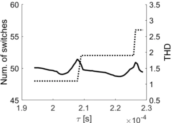
The number of switches per period and the total har- monic distortion (THD) are shown inFig. 11as a func- tion ofτ. The first ONE is staggered. The larger the num-
Figure 7:Reference measurement result
Figure 8:Reference simulation result
Figure 9:Error trajectory during a quasi-steady-state pe- riod
ber of switches is, the greater the switching loss and the smaller the THD are. The optimum is approximately52 switches, therefore,13pulses per period, as is shown in Fig.7andFig. 8. The step concerning the optimal number of switches is magnified inFig. 12.
A local minimum of THD is located at the middle of a staircase (in Fig. 12) when the transient between the positive and negative half periods is smooth as is shown inFig. 13.
By increasingτ, the transients change slightly. First, a V shape appears (seeFig. 14).
By further increasingτ, the V shape transforms into a loop (seeFig. 15) and the last pulses in all half periods have the opposite signs when compared to the reference signal (seeFig. 16) which increases the THD. Finally, the number of switches per period is increased by4and the
Figure 10:The effect ofτon the number of switches
Figure 11:Number of switches and THD as a function of the gradient of the switching line
Figure 12:The optimal number of switches and its THD
transients are in the form of Vs and loops once more (see Fig. 17), which disappear at the middle of the staircase.
4.4 Non-linear load
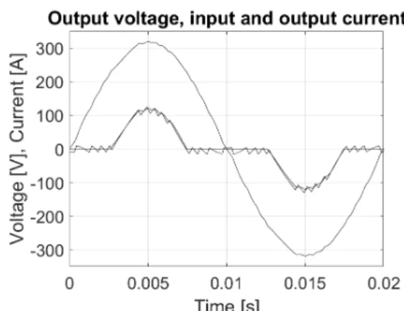
The most challenging load is the rectifier [27], since its current is not sinusoidal and the value of its peak is rela- tively large. A rectifier resembling a load is simulated, which has approximately the same root mean square (RMS) value of the current as that of the nominal cur- rent. The time functions of the output voltage and current in addition to the input current are shown inFig. 18. The RMS value of the input no-load current is zero at the be- ginning of the period, when the output current is zero.
Since the load current is continuous and the reaction of the sliding mode controller is practically instantaneous as a result, this type of non-linear load has no significant ef-
Figure 13:Smooth transient of error trajectory
Figure 14:V-shaped transient of error trajectory
Figure 15:Loop-shaped transient of error trajectory
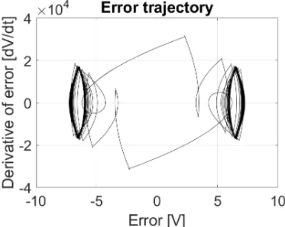
fect on the output voltage - the THD depends on the shape of the error trajectory, which is shown inFig. 19:
4.5 Switching on the load
A nominal resistive load is assumed and the load is switched on at the peak value of the output voltage. The time functions of the voltage and current are shown in Fig. 20. Since the current is discontinuous, a transient is
Figure 16:Control signal
Figure 17:Transient of error trajectory after the number of switches is increased
present, which is recognizable in terms of the shape of the error trajectory inFig. 21. The length of the transient depends on the value ofτ, that is,0.22ms. The transient caused by any step change in the load occurs extremely quickly and only lasts approximately1ms.
5. Conclusions
This paper introduced a follow-up control method with a sinusoidal reference signal for the design of a sliding sur- face and the performance of a Double Relay controller with a dead zone and hysteresis operating in a sliding mode was analysed. The simulation of variable structure systems is very sensitive to the integral method of simu- lation. The zero-crossing must be detected. Even a rela- tively simple controller, which can be implemented by an analogue operational amplifier, also performs very well with a non-linear load. The positive and negative half pe- riods can be separated by a dead zone and the switch- ing frequency limited by hysteresis. The actual number of switches can be set by the gradient of the sliding line.
The value of the THD depends on the shape of the error phase trajectory. A non-linear load with a continuous out- put current has no significant effect on the output voltage because of the instantaneous behavior of the sliding mode controller.
Figure 18:Output voltage as well as input and output cur- rents with a rectifier-like load
Figure 19:Error trajectory of the non-linear rectifier-like load
Acknowledgement
The research reported in this paper and carried out at the Budapest University of Technology and Economics has been supported by the National Research Develop- ment and Innovation Fund (TKP2020 Institution Excel- lence Subprogram, Grant No. BME-IE-MIFM) based on the charter of bolster issued by the National Research De- velopment and Innovation Office under the auspices of the Ministry for Innovation and Technology.
REFERENCES
[1] Utkin, V. I.: Variable structure control optimization (Springer-Verlag), 1992DOI: 10.1007/978-3-642-84379-2
[2] Young, K.: Controller design for manipulator using theory of variable structure systems, IEEE Trans.
Syst. Man Cybern. Syst., 1978,8(2), 101–109DOI:
10.1109/TSMC.1978.4309907
[3] Korondi, P.; Hashimoto, H.; Utkin, V.: Discrete slid- ing mode control of two mass system, in: Proceed- ings of the 1995 IEEE International Symposium on Industrial Electronics, ISIE’95 (Piscataway (NJ), USA), 338–343DOI: 10.1109/ISIE.1995.497019
Figure 20:Output voltage as well as input and output cur- rents after switching on the resistive load
Figure 21:Error trajectory after switching on the resistive load
[4] Korondi, P.; Xu, J., Hashimoto, H.: Sector sliding mode controller for motion control, in: Proceedings of the 8th international power electronics & motion control conference (PEMC, Prague, Czech), 254–
259
[5] Yu, H.; Ozguner, U.: Adaptive seeking slid- ing mode control, in IEEE American Con- trol Conference (Minneapolis, USA), 2006 DOI:
10.1109/ACC.2006.1657462
[6] Chang, E.-C.; Chang, F.-J.; Liang, T.-J.; Chen, J.- F.: DSP-based implementation of terminal sliding mode control with grey prediction for UPS invert- ers, the 5th IEEE Conference on Industrial Elec- tronics and Applications (ICIEA), 2010, 1046–1051
DOI: 10.1109/ICIEA.2010.5515790
[7] Fink, N.: Model reference adaptive control for tele- manipulation,Hung. J. Ind. Chem., 2019,47(1), 41–
48DOI: 10.33927/hjic-2019-07
[8] Young, K.; Özgüner, U.: Frequency shaped sliding mode synthesis, in International Workshop on VSS and Their Applications (Sarajevo)
[9] Fodor, D.; Tóth, R.: Speed sensorless linear param- eter variantH∞ control of the induction motor, in Proceedings of the 43rd IEEE Conference Decision
and Control (IEEE, Piscataway, USA), 4435–4440
DOI: 10.1109/CDC.2004.1429449
[10] Hashimoto, H.; Konno, Y.: Sliding surface design in the frequency domain, in: Variable structure and Lyapunov control , 75–86 (Springer-Verlag), 1993
DOI: 10.1007/BFb0033679
[11] Korondi, P.: Tensor product model transformation- based sliding surface design,Acta Polytech. Hung., 2006,3(4), 23–36
[12] Neukirchner, L. R.; Magyar, A.; Fodor, A.; Kutasi, N.D.; Kelemen, A.: Constrained predictive control of three-phase buck rectifiers,Acta Polytech. Hung., 2020,17(1), 41–60DOI: 10.12700/APH.17.1.2020.1.3
[13] Tai, T.-L.; Chen, J.-S.: UPS Inverter design using discrete-time sliding-mode control scheme, IEEE Trans. Ind. Electron., 2002, 49(1), 67–75 DOI:
10.1109/41.982250
[14] Fedak, V.; Bauer, P.; Hájek, V.; Weiss, H.; Davat, B.; Manias, S.; Nagy, I.; Korondi, P.; Miksiewicz, R.; Duijsen, P.; Smékal, P.: Interactive E-learning in electrical engineering, in: 15th International Con- ference on Electrical Drives and Power Electronics (EDPE) (Podbanské), 368–373
[15] Caceres, R.; Rojas, R.; Camacho, O.: Robust PID control of a buck-boost DC-AC converter, Proc. IEEE INTELEC’02, 2000, 180–185 DOI:
10.1109/intlec.2000.884248
[16] Precup, R.-E.; Preitl, S.: PI and PID controllers tun- ing for integral-type servo systems to ensure ro- bust stability and controller robustness,Electr. Eng., 2006,88(2), 149–156DOI: 10.1007/s00202-004-0269-8
[17] Al-Hosani, K.; Malinin, A.; Utkin, V. I.:
Sliding mode PID control of buck convert- ers, European Control Conference, 2009 DOI:
10.23919/ecc.2009.7074821
[18] Li, H.; Ye, X.: Sliding-mode PID control of DC- DC converter, 5th IEEE Conference on Industrial Electronics and Applications (ICIEA), 2010, 730–
734DOI: 10.1109/ICIEA.2010.5516952
[19] Holtz, J.: Pulsewith modulation - A Survey, IEEE Trans. Ind. Electron., 1992, 39(5), 410–420 DOI:
10.1109/41.161472
[20] Kawamura, A.; Hoft, R.: Instantaneous feedback controlled PWM inverter with adaptive hysteresis, IEEE Trans. Ind. Appl., 1984,20(4), 769–775DOI:
10.1109/TIA.1984.4504486
[21] Aamir, M.; Kalwar, K. A.; Mekhilef, S.: Review:
Uninterruptible power supply (UPS) system, Re- new. Sust. Energ. Rev., 2016, 58, 1395–1410 DOI:
10.1016/j.rser.2015.12.335
[22] Korondi, P.; Hashimoto, H.: Park vector based slid- ing mode control of UPS with unbalanced and non- linear load, in: Variable Structure Systems, Slid- ing Mode and Nonlinear Control (Springer, Lon- don, UK), 193–209DOI: 10.1007/bfb0109978
[23] Korondi, P.; Yang, S. H.; Hashimoto, H.; Ha- rashima, F.: Sliding mode controller for parallel res- onant dual converters, J. Circ. Syst. Comp., 1995, 5(4), 735–746DOI: 10.1142/s0218126695000424
[24] Chang, E.-C.: Study and application of intelligent sliding mode control for voltage source inverters, Energies, 2018,11(10) 2544DOI: 10.3390/en11102544
[25] Széll, K.; Korondi, P.: Mathematical basis of slid- ing mode control of an uninterruptible power sup- ply,Acta Polytech. Hung., 2014,11(3), 87–106DOI:
10.12700/APH.11.03.2014.03.6
[26] Keiel, G.; Flores, J. V.; Pereira, L. F. A.;
Salton, A. T.: Discrete-time multiple resonant con- troller design for uninterruptible power supplies, IFAC-PapersOnLine, 2017,50(1), 6717–6722DOI:
10.1016/j.ifacol.2017.08.1169
[27] Khan, H. S.; Aamir, M.; Ali,M.; Waqar, A.; Ali, S.
U.; Imtiaz, J.: Finite control set model predictive contol for parellel connected online UPS system un- der unbalanced and nonlinear load,Energies, 2019, 12(4), 581DOI: 10.3390/en12040581