´Obuda University

(1)

Obuda University ´

PhD thesis

New adaptive methods for Robust Fixed Point Transformations-based control of nonlinear systems

by

Ter´ ez A. V´ arkonyi

Supervisor:

Dr. J´ozsef K. Tar

Doctoral School of Applied Informatics, ´Obuda University

Budapest, 2013

(2)

(3)

Members of the comprehensive exam committee:

Members of the defense committee:

1. Reviewer:

2. Reviewer:

Day of the defense: 05/24/2013

Signature from head of PhD committee:

(4)

(5)

To my parents who led me through all those years - it must have been a tough job.

And to Fazekas Mih´aly Primary and Secondary Grammar School - well, even black sheep can discolor in time.

(6)

I would like to thank God for his permanent support and that He made all these things possible.

I would like to acknowledge the tremendous help and support of my supervisor, Professor J´ozsef K. Tar. I also would like to thank the guidance and vast help of Professor Vincenzo Piuri.

I would like to thank Professor Imre J. Rudas his great support and encour- age for writing this thesis and that he ensured my working conditions.

I would like to thank the leaders of the Doctoral School of Applied Infor- matics at Óbuda University, Professor Aurél Galántai and Professor László Horváth, and that of the Doctoral School of Computer Science at Univer- sitá degli Studi di Milano, Professor Ernesto Damiani, for giving me the opportunity to take my first steps on the research career.

I also would like to acknowledge the base, the support, and the vast help in the review of my mother, Professor Annamária R. Várkonyi-Kóczy.

I am very grateful of ´Obuda University and Universit´a degli Studi di Milano for the support and the arrangement of the double degree program.

I would like to thank my teachers, Professor József Dombi, Professor András Rövid, Professor Márta Takács, and Professor János Fodor, for giving me insight to new scientific areas during these years.

I am very grateful of Professor Csaba Szab´o for his patience and trust.

Special thanks to Ruggero Donida Labati for the template of the thesis.

Last but not least, I would like to thank my family without whom I could not have written this thesis.

(7)

Introduction

Nowadays, system control is essential in everyday life. It has a long history, e.g. it was applied already by the Romans to handle irrigation systems. In our days, the machines, like mechanical and electronic systems (from the excavators to the CD players) are unimaginable without control.

In the present, as a part of control, one of the most prevalent topics is the control of systems with uncertainties. The growing expectations of avoiding human assistance in situations that need increased attention because of the system’s vagueness or dan- gerousness makes the role of the automated controllers (that can handle vagueness) increased. Just to mention some examples, the automated control of power plants [1], trains [2], or the now-tested “artificial drivers” for cars [3] are like this.

The uncertainties of systems can be divided into three main groups: 1. when the system contains unknown parameters 2. when the system has unknown dynamics 3. when the the system’s state cannot be measured [4]. There are many possible ways how to control such systems, e.g. using as much a priori knowledge as possible, using the linear parametrization method, and/or applying learning mechanisms to gain more information about the uncertainty. After that many controllers can be designed for the system, for example sliding mode controllers [5, 6, 7], fuzzy logic controllers [8, 9], anytime controllers [10, 11], neural network controllers [12, 13, 14], fault tolerant controllers [15, 16], and robust controllers [17, 18]. When the system is not linear in its parameters different adaptive controllers can be designed, like [19].

When the controlled system is just partly known robust controllers bring the most benefit. They have been designed and investigated since the 1950s [20]. Since the first

(12)

applications the area has started a fast progress because the first methods have been sometimes found to lack robustness. The other problem was that in some cases when Sliding Mode Controller, one of first robust controllers [6], was used the actuators have had to cope with high frequency chatter-like control actions that damaged the system. The third reason of the progress was that scientists have realized that robust controllers were very effective when model approximations and disturbances had to be handled in the control process. So the field began to develop. Because of today’s higher expectations the topic is still growing.

One of the recent robust control strategies is the method called Robust Fixed Point Transformations (RFPT). It was first designed to overcome the complexity of Lyapunov function-based techniques for smooth systems [21] but after its robustness was improved [22, 23] it became a powerful technique to reduce the disadvantages of the model approximations and disturbances. The method applies the concept of the so-called expected – realized system response and can be used in the environment of traditional feedback and Model Reference Adaptive control systems [24]. In the first applications it was applied only for single input – single output systems but later it was extended to multiple input – multiple output systems, too [25]. Its aim is to make controllers robust in that case when an approximate model is used to estimate the behavior of the system in the control process. Its great advantage is that it can significantly reduce the errors caused by the model approximation and that the disturbances barely affect its performance.

This thesis focuses on improving RFPT, because though it gives the opportunity to avoid the complexity of Lyapunov’s method, and it can reduce the disadvantages of the model approximation, there are several questions left open and also disadvantages to get rid of because they make uncertain or even limit the usage. The first drawback among them is that RFPT uses the local attraction of a fixed point. The local attraction means that it gains only local stability according to Lyapunov’s stability theorem. This raises the issue if it was possible to achieve its stability.

The other property of RFPT is that theoretically it can improve any existing controller’s results if the control task and the controller meet several conditions. Although, up to this point this statement was proved only for classical controllers. So the question if it could ameliorate other types of controllers is open-ended.

The third aspect which is not to be sneezed at is the applicational possibility in real life. On the one hand, there are fields of application that significantly contribute

(13)

to the improvement of control science. The question is if RFPT could be utilized in these areas. On the other hand, assume that there exists a system or phenomenon which is too complex or some lacking resources (time, knowledge, etc.) do not let it to be modeled accurately. In this case, only a rough approximation of the system can be captured by a model. The main question here is if there is any connection between the analysis of the approximate model and that of the actual system. Is it possible to construct a controller which according to the approximate model’s results can properly control the real system? Will the system reach the desired state accurately enough?

And finally, since Robust Fixed Point Transformations is specialized in approximate models it is possible that it can improve the accuracy of the above mentioned controller so that the model generates truthful output?

The thesis deals with the above questions and gives positive answers to some of them.

The contributions of this thesis can be summarized as follows:

First of all, a new possible application field for Robust Fixed Point Transformations is investigated. Different chaotic attractors are examined and approximate models are built for them. Then RFPT-based controllers are designed for synchronizing two same type attractors based on the built approximate models. The results show that RFPT is appropriate for chaos synchronization because of its robustness: the performance of the original controllers is significantly increased with RFPT, and a well set controller cannot exceed a poorly adjusted controller with RFPT extension.

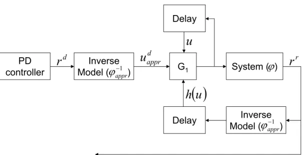
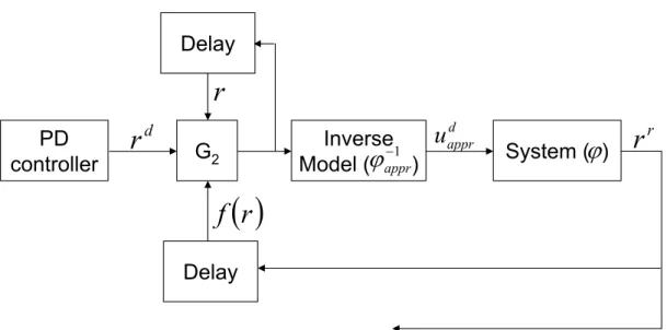
Then the mathematical background of Robust Fixed Point Transformations is analyzed. A new structure for RFPT is proposed in which two controllers are integrated to the system. Then it is shown by illustrative examples that the new structure gains an additional tracking error reduction compared to that of the original methods.

After that, the stability of Robust Fixed Point Transformations is considered. An innovative fuzzy-like parameter tuning method is introduced. It is shown that more stable results of RFPT can be gained if the parameter tuning is applied in the control process.

In the sequel the stability of Robust Fixed Point Transformations is reconsidered.

A new VS-type stabilization algorithm for RFPT is introduced. The results show that when the RFPT-based controller falls out from the local convergence interval it becomes unstable and generates the so-called chattering effect. In the next step it is shown that

(14)

the proposed algorithm can reduce the order of chattering and stops it in very short time. As a consequence the stability of the RFPT-based controllers is gained.

Next the combinability of Robust Fixed Point Transformations is studied. Two types of soft computing (SC) based controllers (Fuzzy Logic Controller and Neural Network Controller) are combined with RFPT then compared to their original form.

The results verify that the robustness of the controllers can be increased with the application of RFPT and by this the error produced by the original soft-computing- based controllers can be reduced significantly.

Afterwards, the applicability of Robust Fixed Point Transformations is investigated.

A hydrodynamic model of freeway traffic is studied from the viewpoint of stability. The stationary solutions of the model are determined and their stability is analyzed. Then an RFPT-based controller is designed to control the emission rate of exhaust fumes for the stationary solutions. Finally, the effectiveness of the controller is examined by comparing its results to the same controller without RFPT.

Finally, preliminary investigations are made for a possible anti-lock braking system.

A simple approximate model and a controller is designed for an anti-lock braking system. Then the results show that though the system of a vehicle can be approximated roughly with the proposed model, good results can be obtained with the suggested controller.

The analysis testifies that RFPT can be applied in several areas successfully. The investigations also prove that the contributions suggested by the author improve the performance of the RFPT-based controllers and avoid several of their disadvantages.

First it is shown in Chapter 5 that RFPT can be successfully applied in the field of chaos synchronization. Secondly the new structure proposed in Chapter 6 reduces the tracking errors achieved by the original versions of RFPT. Thirdly the two innovative methods introduced in Chapters 7 and 8 make the RFPT-based controllers stable. Fourthly in Chapters 9 and 10 two types of soft-computing-based controllers are combined with RFPT. Finally, in Chapters 11 and 12 a real and a possible aspect of real application of RFPT are shown: first, a hydrodynamic model of freeway traffic is analyzed in the viewpoint of stability and controlled with RFPT-based controller, then a simple model for an anti-lock braking system is designed and controlled without RFPT, but with the possibility of the extension. The constructed models make sure that there is a

(15)

huge difference between the systems and their approximate representatives and that controlling them with RFPT-based controllers can bring results that reflect to reality.

The thesis is organized as follows. First, in Chapter 2 some classical controllers are reviewed that use Lyapunov function for control or parameter tuning. In Chapter 3 some nonlinear systems are introduced that are applied to help the analysis of the worked out methods by simulations. In Chapter 4 the basics of Robust Fixed Point Transformations are shown. In Chapter 5 the effectiveness of RFPT in chaos synchronization is investigated. Chapters 6-8 contain the improving extensions for RFPT: the new structure, the fuzzy-like parameter tuning and the VS-type stabilization method, respectively. Chapters 9-10 present two prevalent soft computing-based families of controllers that are extended with RFPT. In Chapters 11 and 12 two realistic phe- nomenons are modeled, controlled, and parsed: in the prior with-, in the latter without RFPT (but with the possibility of the extension). The last chapter deals with the final conclusions.

(16)

(17)

2

State of the art

In Chapter 1 the development of nonlinear control theory and some open questions of the field are summarized. In this chapter, the emphasis is put on those methods that form the basis for the new ideas of this work. First, Lyapunov Stability Theory is briefly explained, then some traditional controllers are introduced and finally, two soft computing techniques are detailed that can advantageously be used for control purposes.

2.1 Lyapunov Stability Theory

In the first part of the 19^th century, stability of nonlinear systems was a problematic subject for the scientists. Only a few results were at hand to answer the question weather a system is stable or not. The first major aid came from Aleksandr Lyapunov in 1892 [26, 27]. In his dissertation he introduced his stability theory and an approach called Lyapunov’s second or “direct” method in which he showed a way how to determine a nonlinear system’s stability without solving its equations of motion. Since most of the problems appearing in real life do not have analytical solutions in closed form and the numerical solutions are valid only with time limitation, Lyapunov’s method brought a breakthrough for the field of control. His development proved to be so significant that the stability of most of the controllers is ensured by his “direct” method even in our days.

Assume a dynamic system described by a set of ordinary differential equations expressing by arrays as

(18)

˙

x=f(x, t) (2.1)

where x ∈ Rⁿ, t ∈ [t₀,∞), and x(t₀) = x₀. Let x denote some tracking error (in this case the main goal is to keep x as close to 0 as it is possible). If it is known that the system has one unique solution, according to Lyapunov Stability Theorem the followings can be stated:

• Point x^∗ ∈Ris an equilibrum point of the system if ∀t∈[t₀,∞) f(x^∗, t) = 0.

• Equilibrum x^∗ is locally stable if every solution that starts close to x^∗, remain close tox^∗ and asymptotically stable if in addition the solutions tend towardsx^∗.

• Equilibrumx^∗ is stable int=t₀ if∀ǫ >0 ∃δ(ǫ, t0)>0 such thatkx(t0)−x^∗k<

δ=⇒ kx(t)−x^∗k< ǫ,∀t > t0.

• Uniformly stable equilibrums can be defined if in the above definitionδ depends only on ǫ.

• Equilibrumx^∗ is asimptotically stable att=t₀ if it is stable and∃δ(t0)>0 such thatkx(t0)−x^∗k< δ=⇒ kx(t)−x^∗k →0 fort→ ∞.

• Equilibrumx^∗ is globally stable if it is stable for every initial conditionx₀∈Rⁿ. To be able to determine whether system (2.1) is stable or not, there are two choices.

The first option is integrating and solving (2.1) explicitly. This solution is applicable only in some special cases. Thanks to Lyapunov’s direct method there is an other option. Instead of solving the equation, a uniformly continuous and positive definite function V can be constructed with a non-positive time-derivative on the domaint ∈ [0,∞) which can be used to prove the stability of the controller. This function can be calculated based on the tracking errors and the modeling errors of the system’s parameters. According to the Barbalat lemma (stating that if a function^dV_dt is uniformly continuous and its integralV(t) is bounded then the function itself converges to zero as t→ ∞) [28] the derivative ofV converges to zero. As a result, the tracking errors and the modeling errors have to remain bounded or in a special case they have to converge to zero.

(19)

2.2 Classical controllers

To show that function V is bounded, a function classK is introduced that can be used as upper and lower bounds of function V. Function κ : [0, k) → [0,∞) where k <∞is a member of classK ifκ(0) = 0 andκ(t) is strictly increasing. Let us assume thatα(kxk), β(kxk), andγ(kxk) belong to function classK. In this case according to Lyapunov’s second method it can be stated that

• IfV(0, t) = 0 and∀x∈Bǫ(0) (whereBǫ(0) denoted theǫvicinity of 0) and∀t≥0:

V(x, t) ≥ α(kxk) > 0 and ˙V(x, t) ≤ 0 holds locally in x and for all t, then the equilibrum pointx= 0 is locally stable.

• If V(0, t) = 0 and V(x, t) ≥ α(kxk) > 0 and ˙V(x, t) ≤ 0 then the equilibrum pointx= 0 is stable.

• IfV(0, t) = 0 andV(x, t)≥α(kxk)>0 and ˙V(x, t)≤0 andV(x, t)≤β(kxk)>0 then the equilibrum pointx= 0 is uniformly stable.

• IfV(0, t) = 0 andV(x, t)≥α(kxk)>0 and ˙V(x, t)≤0 andV(x, t)≤β(kxk)>0, and ˙V(x, t)≤ −γ(kxk) then the equilibrum point x= 0 is uniformly asymptotically stable.

2.2 Classical controllers

In this section, four classical controllers are discussed that are strongly related to the focus of this work. First the PID controller is shown in details which has been developed parallel with Lyapunov’s method. Then the Computed Torque Control (CTC) and its special case, the Adaptive Inverse Dynamics are summarized together with a simple example. The example includes the proof of the controller’s (Lyapunov) stability. Finally, the Model Reference Adaptive Controller, an illustrating example, and the Lyapunov stability proof are shown.

2.2.1 Proportional-Integral-Derivative Controller

The Proportional-Integral-Derivative (PID) controller was introduced in 1911 [29]. It was first used for automatic ship steering. It has become the most common feedback controller in the industry. In the industry, most of the machines are supervised by PID

(20)

Σ

P

I

D

Σ

^System



^t

 

i e d

K

0



 

dt t K_d de

 

^t

e K_p

e(t)

+ +

-

y_ref(t) u(t) y(t)

Figure 2.1: The block scheme of the traditional PID Controller.

controllers. This control strategy is popular because of its simplicity and easy handling.

It can be described by

u(t) =K



e(t) + 1 Ti

t

Z

0

e(τ)dτ+Td

de(t) dt



 (2.2)

where u denotes the control signal, e = yref −y marks the tracking error, y stands for the output and y_ref for the desired output of the controlled system; t is the time.

K, Ti, and Td denote the free variables of the controller. For simplicity the notations Kp := K, Ki := _T^K

i, and Kd := KTd are also commonly used. The block diagram of the traditional PID controller is shown in Fig. 2.1.

Special cases of PID controller are also widely used nowadays. If one or two of the three parameters in (2.2) are set to zero, similar controllers can be gained like PD, PI, I, etc. controllers.

There are many possibilities for tuning the parameters of the PID controller. One of the most popular tuning strategies, called frequency response method has been developed by Ziegler and Nichols, see [30]. The essence of the tuning is the following:

setKi andKd zero and increaseKp until the controlled system starts to oscillate. Let S_u denote this (high) value of K_p and P_u denote the oscillation period of the system.

In this case, the proposed values for the parameters are Kp = 0.6Su, Ki = 2^S_P^u

u, and K_d= ^S^u₈^P^u.

(21)

There are other possibilities how to determine the parameters, though they are not used any more in the industry. Instead of them PID tuning and loop optimization softwares are applied to ensure stable and good results (see e.g. [31]).

In the following, a simple example is shown how to determine numerically the parameters of a PID controller which controls a damped string described by the following equation:

¨

x=−kx−bx˙+cu (2.3)

where x stands for the system state variable, k, b, and c are free parameters, and u denotes the control force. If a certain behavior is prescribed for the system by a reference model

¨

x^Ref =−kx^Ref−bx˙^Ref+cu (2.4) where the meaning of the parameters are the same, then the proper control force for the system can be calculated as

u= 1 c

x¨^Ref+kx^Ref+bx˙^Ref

(2.5) The PID correction can be added to (2.5) as

u= ¹_c x¨^Ref+kx^Ref+bx˙^Ref + P x^Ref−x

+D x˙^Ref−x˙ +I

t

R

0

x^Ref−x

dτ (2.6)

If (2.6) is substituted to (2.3) then after restructure the following equation is gained:

¨

x^Ref−x¨=−(k+cP)(x^Ref−x)−(b+cD)( ˙x^Ref−x)˙ −cI

t

Z

0

(x^Ref−x)dτ (2.7) Ifh=x^Ref−x denotes the error, then after a derivation (2.7) takes the form of

...h =−(k+cP) ˙h−(b+cD)¨h−cIh (2.8) Leth=e^αt. In this case,

α³ =−(k+cP)α−(b+cD)α²−cI (2.9)

(22)

from which

α³+ (k+cP)α+ (b+cD)α²+cI = 0 (2.10) is gained. Let α₁,α₂, and α₃ denote the roots of (2.10). It can be stated that

k+cP =α₁α₂+α₂α₃+α₁α₃ cI =−α1α2α3

b+cD=−α1−α₂−α₃

(2.11) In the knowledge ofα₁,α₂, andα₃, the parameters of the PID controller can be set so that (2.8) converges to 0.

Despite the popularity of the PID controllers, they can be applied only if the controlled system is transparent and the effects of the feedback of the PID controller can be followed qualitatively. If not, then the controller cannot achieve optional system behavior. For example, if the pendulum of a cart-pendulum system (see Chapter 3) passes through the horizontal line, the behavior of the system changes and the control law determined by the PID controller will not be valid for the system any more. As an example for proper systems, the damped strings could be mentioned, because they are qualitatively transparent and they can be used as approximate models for many control problems, e.g. for stabilization tasks around an operating point.

2.2.2 Computed Torque Control (CTC) and the adaptive inverse dynamics control

The Computed Torque Control [32] is a control strategy usually applied on robots. The most important property of relatively simple robots is that they can be described ana- lytically, so a relationship can be established between the joint coordinate accelerations and the torques or forces acting on the system (the forces and torques are made partly by the robot’s own drives and/or by its environment with which the system may be in dynamic coupling). The relationship is described by the so-called Euler-Lagrange equations of motion:

H(q)d²q dt² +h

q,dq

dt

=Q (2.12)

whereH(q) denotes the inertia matrix of the system, a part of h(q,q) is quadratic in˙

˙

q and describes e.g. the Coriolis terms, while its other part depending only on q is

(23)

responsible for the gravitational effects. Due to physical reasonsHis always symmetric and positive definite. The termQ stands for the generalized forces of the robot’s own drives and the environment, e.g. forces for the prismatic generalized coordinates, and torques for the rotational axes. In the possession of this model (on the basis of purely kinematic considerations) some desired ^d²_dt^q^des₂ can be computed in each control cycle to exert the necessaryQ^des. This part of the controller is often referred to as “feedforward”

control. For more precise tracking the “feedforward part” generally has to be completed by PID-type feedback terms based on the tracking error.

An important practical problem of CTC is that in many cases it is very difficult (or even impossible) to identify the parameters of the analytical models of the systems (see e.g. the model for the six degree of freedom PUMA robot [33], where the model construction took five weeks for three persons). Another practical problem in the application of this method is that normally there are no sensors available that could exactly measure the external (e.g. environmental) parts that affect Q. Their effects can be observed only subsequently and generally cannot efficiently be compensated by simply prescribing some feedback correction in ^d²_dt^q^des2 .

If the kinematic model of the system is precisely known, the Adaptive Inverse Dy- namics Control can be a solution. Letprepresent the dynamical parameters (unknown) and Y

q,^dq_dt,^d_dt²^q2

the array built up based on the kinematic functions (known). The dynamic model can be formulated as

H(q)¨q+h(q,q) =˙ Q=Y(q,q,˙ q)p¨ (2.13) It is supposed that some approximation for H(q), h(q,q), and˙ p are available as H(q),ˆ ˆh(q,q), and˙ p. The exerted forces may contain feedback-correction dependingˆ on the tracking error and its derivativese=q^des−q, ˙e=q˙^des−q, and˙ ¨e=¨q^des−¨q, with some symmetric positive definite gain matrices K₀ and K₁. In this case

H(q)(¨ˆ q^des+K₀e+K₁˙e) +ˆh(q,q) =˙ Q=H(q)¨q+h(q,q)˙ (2.14) It is assumed that Q originates from the drives and does not contain unknown external components, so by subtracting (2.14) from (2.13) we can obtain

H(q)¨q+h(q,q)˙ −H(q)(¨ˆ q^des+K₀e+K₁˙e)−ˆh(q,q) = 0˙ (2.15)

(24)

and then by subtracting with Hˆ (q)q¨ and reordering H(q)(¨ˆ e+K₀e+K₁˙e) =

H(q)−H(q)ˆ

¨ q+

h(q,q)˙ −ˆh(q,q)˙

=Y(q,q,˙ ¨q) (p−ˆp) (2.16) where the left hand side contains the model data, while the other side contains the modeling errors: H˜ :=H(q)−H(q),ˆ h˜:=h(q,q)˙ −hˆ(q,q), and˙ p˜:=p−ˆp. Via multi- plying both sides with the inverse of the known model, the following standard form is obtained:

˙e

¨ e

−

0 I

−K0 −K1

e

˙e

= 0

Φ˜p

(2.17) whereΦ=Hˆ⁻¹(q)Y(q,q,˙ ¨q).

Let us introduce the following notations: x :=

e

˙e

, x˙ :=

˙e

¨e

, B :=

0 I

, and A=

0 I

−K0 −K1

. By this, the system can be described in a more simple form:

˙

x−Ax=BΦ˜p (2.18)

For the tracking error e, the first derivative of it ˙e, and the parameter estimation errorp˜ the following Lyapunov functionV can be constructed:

V =x^TPx+˜p^TR˜p (2.19)

whereP andR are constant, symmetric positive definite matrices. In this case V˙ =x˙^TPx+x^TP ˙x+p˙˜^TR˜p+p˜^TR ˙˜p<0 (2.20) From (2.18) it follows that

V˙ =x^T A^TP+PA

x+p˜^TΦ^TB^TPx+x^TPBΦ˜p+p˙˜^TR˜p+p˜^TR ˙˜p<0 (2.21) Due to the symmetry of matricesP andR (2.21) can be simplified as

V˙ =x^T A^TP+PA

x+2˜p^TΦ^TB^TPx+2˜p^TR ˙˜p<0 (2.22) To guaranteedV /dt <0 for any finitex, the following restrictions can be prescribed:

let U be a negative definite symmetric matrix, and let

(25)

A^TP+PA=U (2.23)

further

˜ p^T

Φ^TB^TPx+R ˙˜p

=0⇒p˙˜=−R⁻¹Φ^TB^TPx (2.24) where (2.23) is referred as Lyapunov equation. Normally an appropriateUis prescribed and the task is to find a proper Pfor this U by solving the Lyapunov Equation. The Lyapunov Equation sets linear functional connection between the elements of P and U that may or may not have solution. (For the existence of a solution the real part of each eigenvalue ofA must be negative.) SinceA=constant, the Lyapunov Equation has to be solved only once in order to find a properPfor the prescribed U. To satisfy the second constraint (2.24), its right hand side has to be expressed from its definition through Band Φ. It is obtained that

˙˜

p=p˙ −p˙ˆ =−R⁻¹Y ˆH⁻¹[0,I]Px (2.25) in which the computational burden mainly consists of the need for inverting the model inertia matrix that must have the exact, intricate form determined by the particular kinematic model of the given system.

If the adaptation rule is applied, then the following cases can be separated:

• If kxk → 0 and k˜pk > F > 0 then exponential trajectory tracking is achieved without exactly learning the system model.

• If kxk → 0 and k˜pk → 0 then exponential trajectory tracking is achieved with exactly learnt system model.

kxk> E >0 for arbitrarily long time is not possible since an initially finite positive valueV(0) with at least constant speed of decrease has to achieve 0 during finite time.

2.2.3 Model Reference Adaptive Controller

The Model Reference Adaptive Controller (MRAC) belongs to the family of direct adaptive controllers [34]. It was proposed in 1958 to control an aircraft driven by a joystick [35]. It had stability problems during the first few years until Lyapunov

(26)

functions have been started to be used for the design. The first successes were reached in 1966 [36, 37].

MRAC is based on the idea of constructing a reference model that determines the desired behavior of the system. Then the control signal is calculated by the difference of the model’s and the system’s output (tracking error). Its structure is very simple, having four main parts:

• The system: it has known structure but contains unknown parameters. For nonlinear systems it can be said that the structure of the nonlinear equations are known, but some of the parameters are not.

• The reference model: it specifies the desired output of the controlled system.

It has to be designed parallel with the controller. Further, it has to reflect the performance specification (like rise and settling time, overshoot, etc.) and its output has to be achievable for the system (e.g. its order and relative degree have to match the system’s assumed order and degree).

• The feedback controller (or control law): it is parameterized by adjustable parameters. If the system parameters are all known, it has to force the system to act exactly like the reference model (prefect tracking). If the system parameters are not known, it has to achieve perfect tracking asimptotically.

• An adaptation law: it is used to adjust the parameters of the controller. The goal is to set the parameters so that the system’s output equals the model’s output.

The main issue of the MRAC design is to ensure that the controller remains stable and the tracking error converges to zero.

The block scheme of the traditional MRAC is shown in Fig. 2.2.

For designing a Model Reference Adaptive Controller, as an example, consider the system assumed in [5]. In this very simple system a massm is settled on a frictionless surface and controlled by a motor: m¨x = u, where u denotes the force of the motor and x is the position of the mass. The positioning commands r(t) come through a joystick handled by a human. In [5] the following reference model is suggested:

¨

x^m+λ₁x˙^m+λ₂x^m =λ₂r(t), wherex^mis the output of the reference model. Parameters λ₁ and λ₂ (λ₁, λ₂ > 0) are chosen to reflect the performance specifications of the systems.

(27)

2.3 Soft computing techniques

Reference Model

System Controller

Adaptation Law

u y

y^m

Figure 2.2: The block scheme of the traditional Model Reference Adaptive Controller taken from [38].

If the mass m is known, perfect tracking is achieved by the control law u = m x¨^m−λe˙−λ²e

, where e = x(t)−x^m(t) and λ is strictly positive. So the expo- nentially convergent tracking error dynamics are ¨e+ 2λe˙+λ²e= 0.

If the mass is not known exactly, the applied control law isu= ˆm x¨^m−λe˙−λ²e , where ˆm is adjustable. Let bes= ˙e+λe, v = ¨x^m−2λe˙−λ²e, ande_m = ˆm−m. In this case, the error dynamics arems˙+λms=emv. The parameter adjustment for the mass is ˙ˆm=−γvs, whereγ is called the adaptation gain, and it is a positive constant.

The stability analysis of the above explained controller can be shown by Lyapunov’s theory. Consider the following function V = ¹₂

ms²+ ¹_γe²_m

as a Lyapunov function for the system, where ˙V = −λms². With the help of the Barbalat lemma it can be proven thats converges to zero which indicates the trajectory and velocity tracking.

2.3 Soft computing techniques

In this section, two important soft computing techniques are summarized that can advantageously be used in the control area: the fuzzy theory and the field of neural networks. Both are relevant and getting more popular as the control tasks include more uncertainties and lack of knowledge.

2.3.1 Fuzzy Theory

Fuzzy control methodologies have emerged in recent years as promising tools to solve nonlinear control problems. The fuzzy approach was first proposed by Lotfi A. Zadeh,

(28)

in 1965 when he presented his seminal paper on fuzzy sets [39]. Zadeh showed that fuzzy logic unlike classical logic can handle and interpret values between false (0) and true (1). One of the most successful application areas of Fuzzy Logic proved to be Fuzzy Logic Control (FLC), because FLC systems can replace humans for performing certain tasks, for example control of a power plant [1], or aeroelastic wing section [11], etc. [40, 41, 42].

An other significant reason for applying fuzzy techniques in control is their simple approach which provides to use heuristic knowledge for nonlinear control problem.

In very complicated situations, where the plant parameters are subject to perturba- tions or when the dynamics of the systems are too complex to be described by exact mathematical models, adaptive schemes have to be used to gather data and adjust the control parameters automatically. Based on the universal approximation theorem [43] and by incorporating fuzzy logic systems into adaptive control schemes, a stable fuzzy adaptive controller is suggested in [44] which was the first controller being able to control unknown nonlinear systems. Afterwards, a wide variety of adaptive fuzzy control approaches have been developed for nonlinear systems, like [45, 46, 47]. In the following the basics of Fuzzy theory are summarized.

2.3.1.1 Definitions

Definition 1 (Universe). A fuzzy universe is the domain of the observations. Values, objects that need to be classified.

Definition 2(Linguistic value). Linguistic values are words, symbols (sets) defined by the rate of belonging of the elements of the universe.

Definition 3 (Linguistic variable). A linguistic variable is an overall notion with the help of which the linguistic values in a specific topic can be referred.

Definition 4 (Membership function). Membership function is a mapping expressing the rate of belonging of a universe element to a linguistic value.

Definition 5(Fuzzy set). Fuzzy set is a set to the elements of which a number between 0 and 1 can be assigned. The assignment is the membership function. IfAis a fuzzy set over universe X, then µA(x) :X→[0,1] is the membership function of setA. In case of discrete sets A =

n

P

i=1

µA(xi)/(xi) denotes the fuzzy set A, where xis are elements of X, with µA(xi) membership value (in set A). In continuous case the notation is A=R

XµA(x)/x, where x∈X andµA(x) is its membership value in set A.

(29)

Definition 6 (Height of a fuzzy set). The height of fuzzy set A on universe X is hgt(A) = sup

x∈X

µA(x). The fuzzy sets with height=1 are called normalized fuzzy sets.

The fuzzy sets with height<1 are called subnormal fuzzy sets.

Definition 7 (Core). The core of fuzzy set A on universe X is crisp subset of A:

core(A) ={x∈X|µA(x) = 1}.

Definition 8 (Support). The support of fuzzy set A on universe X is crisp subset of A: supp(A) ={x∈X|µA(x)>0}.

Definition 9 (α-cut). The α-cut of fuzzy set A on universe X is crisp subset of A:

α−cut(A) = {x ∈ X|µA(x) ≥ α}. The core of A can also be defined as core(A) = 1−cut(A).

Definition 10 (Strongα-cut). The strong α-cut of fuzzy set Aon universe X is crisp subset of A: α−cut(A) = {x∈ X|µA(x)> α}. The support of A can also be defined as supp(A) = 0−cut(A).

Definition 11(Convex fuzzy set). The fuzzy setAon universeXis convex if∀x1, x₂, x₃ ∈ X,x₁≤x₂ ≤x₃ →µ_A(x₂)≥min(µ_A(x₁), µ_A(x₃)).

Definition 12 (The normalization of a fuzzy set). The normalization of fuzzy set A on universeX results in an other (normalized) fuzzy setA^′ for whichµA^′(x) = _hgt(A)^µ^A^(x)), x∈X.

Definition 13 (Fuzzy subset). The fuzzy set B is subset of fuzzy setA on universeX if ∀x∈X µA(x)≤µB(x)

Definition 14(Fuzzy partition). Fuzzy partition means the partitioning of the universe by linguistic variables. Let A₁, A₂, ..., AN denote fuzzy subsets of universe X so that

∀x∈X

NA

P

i=1

µAi(x) = 1, whereAi 6=∅, and Ai 6=X. In this case the set consist of fuzzy sets Ai is a fuzzy partition.

Definition 15 (Fuzzy number). The fuzzy set A on universe X (in most of the time X = R) is a fuzzy number, if A is convex and normalized, µa(x) is semi-continuous and the core ofA contains only one element.

Definition 16 (Fuzzy interval). The fuzzy set A on universe X is a fuzzy interval, if A is convex and normalized, and µa(x) is semi-continuous.

(30)

2.3.1.2 Operations on fuzzy sets

The intersection and union operations defined by Zadeh in 1965 are the following. For the intersection:

µ_A∩B = min (µ_A(x), µ_B(x)) For the union:

µ_A∪B= max (µA(x), µB(x))

Since then, various definitions have been developed, like the T-norms, T-conorms, and the S-norms that all fulfill some given axioms.

Definition 17 (T-norm). T-norm T is a mapping T : [0,1]×[0,1]→ [0,1], with the following constraints:

T-1 T(a,1) =a

T-2 b≤c⇒T(a, b)≤T(a, c) T-3 T(a, b) =T(b, a)

T-4 T(T(a, b), c) =T(a, T (b, c))

The T-norms also satisfy the following condition: TW(a, b)≤T(a, b)≤min(a, b), where T_W(a, b) =











a b= 1 b a= 1 0 otherwise

is called Weber T-norm [48].

Definition 18 (T-conorm). T-conorm S is a mapping S : [0,1]×[0,1]→ [0,1], with the following constraints:

S-1 S(a,0) =a

S-2 b≤c⇒S(a, b)≤S(a, c) S-3 S(a, b) =S(b, a)

S-4 S(S(a, b), c) =S(a, S(b, c))

(31)

The T-conorms also satisfy the following condition: max(a, b) ≤ S(a, b) ≤SW, where S_W(a, b) =











a b= 0 b a= 0 1 otherwise

is called Weber S-norm (T-conorm) [48].

Definition 19(Fuzzy complement). The complement defined by Zadeh isc(a) = 1−a.

The complementA of fuzzy set A can be defined by as follows

c-1 c(0) = 1

c-2 a > b⇒c(a)< c(b) c-3 c(c(a)) =a

Definition 20 (Fuzzy reasoning). Fuzzy logic can be deduced from fuzzy set theory just as classical logic from classical set theory. The operations “and”, “or”, and “not”

correspond to “intersection”, “union”, and “complement”, respectively. Fuzzy logic is built on sets enabling the predicates to be linguistic variables.

Statement - Fuzzy statements are simple statements with linguistic labels of fuzzy sets combined by “and”, “or”, and “not”.

Implication - Fuzzy implications can be defined in many ways (just like in the classical case), but result in different outputs depending on the chosen T- and S-norms.

2.3.1.3 Rule-based fuzzy reasoning

The block scheme of the rule-based fuzzy reasoning system can be seen in Fig. 2.3. The input (observation), and the output (conclusion) are usually not fuzzy-type quantity.

The transformation between the crisp values and the fuzzy sets is made by the fuzzification, and defuzzification blocks. The deduction is made by the reasoning block using the a priori knowledge of the given rule base. The reasoning block determines how much each rule is valid for the concrete input. In case of multiply inputs the validity is determined by the “weakest” input. Then the conclusion is calculated.

Fuzzification - The fuzzifying block transforms a crisp input to a fuzzy set. The most often used technique is the singleton fuzzification (the membership function is 1 at the input, and 0 otherwise). Less simple, but closer to reality is if the uncertainty and accuracy of the input is illustrated and the input is transformed

(32)

to e.g. a fuzzy number. The uncertainty can principally be represented by an α-cut.

Rule base - The rules give the basics of the rule-based fuzzy systems. The rule base describes the a priori knowledge on the system. The rules are usually “IF...

THEN...” type rules. The i^th rule can be expressed as

R_i :IFx₁ is X_i,1 and x₂ isX_i,2 and . . . and x_n isX_i,n THEN y₁ is Y_i,1 and . . . and ym isYi,m.

wherex₁, ..., xnare inputs withX_i,1, ..., Xi,nlinguistic values,y₁, ..., ymare output variables withYi,1, ..., Yi,1m linguistic values.

Reasoning - According to the reasoning strategy two main rule-based systems can be determined: the composition-based reasoning, which determines its output as the compositionX◦R; and the individual rule-based reasoning, which determines the output (Y^′) as the union of the composition of the inputs and the individual rules. The prior is the one based by fuzzy theory, but the latter provides less computational time this is why the individual rule-based reasoning is more prevalent.

Defuzzification - Defuzzification is responsible for the transformation of the fuzzy outputs to crisp values. Various methods are known depending on the output fuzzy set, but the most prevalent approaches are the center of area (CoA), the center of gravity (CoG), the center of maxima (CoM), and the mean of maxima

fu zz if i cation d ef u z zi fi cation

Fuzzy reasoning

input output

Figure 2.3: Fuzzy reasoning, taken from [49].

(33)

(MoM) defuzzification methods. As an example, the CoG defuzzification can be calculated as

y^′= R

Y^′

µY^′(y)ydy R

Y^′

µ_Y′(y)dy (2.26)

for continuous values, and

y^′ =

Ni

P

i=1

µY^′(yi)yi Ni

P

i=1

µ_Y′(yi)

(2.27)

for discrete values, where Ni denotes the number of the discrete values with the help of which µY^′(y) membership function can be discretized.

2.3.2 Artificial neural networks

Human recognition and control abilities far exceed those of complex intelligent control systems (e.g. robots). This has motivated scientist to analyze the human thinking to model neurons and nervous systems and use artificial neural networks in many areas (e.g. image precessing, signal processing, and control) [50]. The basic idea is according to natural neural networks to construct artificial systems (nets) consist of similar in- terconnected units (neurons). Though, the artificial neurons and neural networks are sketches compared to the natural ones, they have some important similar abilities, e.g.

parallel processing, modularity, fault tolerance, and the ability to learn. The parallel synthesis shortens the computational time and makes sure that several disabled units do not influence the performance of the net considerably.

Neural networks are very helpful in classification, recognition problems, and optimization problems. In the thesis only feedback neural networks are used with backpropagation. The followings are valid mainly for this type of neural networks.

2.3.2.1 The structure of the neural networks

Neural networks are information processing tools characterized by parallel processing and a learning algorithm. Their unit is an artificial neuron with multiple inputs, one processing function, one output, and local memory. The easiest and most common type

(34)

of neuron is a perceptron which calculates its output by a nonlinear transform of the weighted sum of the inputs (see Fig. 2.4)

y=f

N

X

i=0

wixi

!

=f w^Tx

(2.28) where x= [x0, x1, ..., xN]^T,w= [w0, w1, ..., wN], xi are input scalars with wi weights, and the weighted sum iss. The value ofx₀, called bias, is usually a nonzero constant.

The nonlinear map is denoted by f, while y marks the output of the neuron. For determining the nonlinear map, many strategies can be found in the literature, like the binary transfer function

y(s) =

(+1 s >0

−1 s≤0 (2.29)

the piecewise-linear transfer function

y(s) =







+1 s >1 s −1≤s≤1

−1 s <−1

(2.30)

and the sigmoid transfer function

y(s) = 1−e^−Ks

1 +e^−Ks;K >0 (2.31) The three example functions are shown in Fig. 2.5.

w

1

w

0

w

2

w

n 0

1 x

x

1

x

2

x

n

s

f y f (s )

¦

Figure 2.4: The scheme of a neuron without memory, with equal inputs, taken from [49].

(35)

2.3.2.2 Topology of the neural networks

The topology of a given neural network is how it is structured, e.g. where its in- and outputs are. The NNs are usually presented by directed graphs, where the nodes represent the neurons and the weighted edges denote the weighted connections. The neurons can be divided in three groups: input neurons (input of the network), output neurons (output of the network), and hidden neurons (inputs and outputs of other neurons in the network). They can be organized in layers, where each layer contains the same type of neurons. Thus, three different type of layers can be defined: input layer, output layer and hidden layer. The output of the input layer and the hidden layers are connected to other hidden layers or directly to the output layer. If the graph representation of the neural network contains a loop, it is called feedback neural network. Otherwise it is called feedforward neural network.

2.3.2.3 MultiLayer Perceptron

The most common multilayer feedforward neural network is the MultiLayer Perceptron (MLP) [51], where the connections are only between neighboring layers. The weights of the connections produce the free parameters of the NN. An example for an MLP is shown in Fig. 2.6. The example hasN+ 1 inputs (x¹₀, x¹₁, ..., x¹_n), two hidden layers with three and two neurons, and two outputs (y1, y2). The weight matrices are denoted by W⁽¹⁾ and W⁽²⁾ while the biases for the layers are marked byx¹₀ and x²₀. The applied transfer function is the sigmoid one.

s )

(s y

1 1

s )

y(s

1 1

s )

(s y

1 1

Figure 2.5: Typical nonlinearities in neurons: binary (left); piecewise-linear (middle);

sigmoid (right).

(36)

¦

^sgm

¦

^sgm

¦

^sgm

¦

^sgm

¦

^sgm

¦

) 1

1 (

x0

) 1 (

x1

) 1 (

x2

) 1 (

xn

) 1

W(

) 1 (

s1

) 1 (

s2

) 1 (

s3

) 1 (

y1

) 1 (

y2

) 1 (

y3 ) 1

2 (

x0

) 2 (

s1

) 2 (

s2

y1

y2

d1

d2

H2

H1

) 2

W(

Figure 2.6: An example for a multilayer perceptron, taken from [49].

2.3.2.4 Supervised training

The desired behavior of the neural network is gained by the tuning of the weights which is called training. An appropriately complex neural network can be considered as an universal approximator, however achieving z optimal weight is an NP-complete problem to the training algorithms can give only near optimal results.

Figure 2.7 shows the general scheme of the training, where the expected coherent input-output pairs are given. In case of supervised training the output of the network can be compared to the desired output. From the comparison an error can be calculated which is used to modify the training in the proper way (through a criteria function or a parameter tuning algorithm).

2.3.2.5 Training one perceptron

The weight modification can be done by the least mean square (LMS) algorithm the criteria of which is the square of the actual error (see Fig. 2.8):

s=w^Tx y=sgm(s)

ǫ=d−y

(2.32)

(37)

Unknown system

Model g( , )u n

g’( , )u n

u

n

d

C

y

Param te r modificatione algorithm

Criteria function C(d,y)

Figure 2.7: The block scheme of the training, where u the independent variables, n stands for the noise signals, andCmarks the criteria function (usually a least mean square function), taken from [49].

wheredis the output of the real system,y is the output of the network, andǫdenotes the actual error. Functionsgm stands for the nonlinear transfer function. The actual error can be expressed in more details:

+1

-1

Param ter e modification algorithm

x₀=1

w₁(k)

w_N(k) xN(k)

w₀(k)

x₁(k)

x(k) s(k)

y(k)

d(k) -

İ(k) + 6

6

Figure 2.8: An illustrative example for modifying the weights of a neuron, taken from [49].

(38)

ǫ(k) =d(k)−y(k) =d(k)−sgm(s(k)) =d(k)−sgm w^T(k)x(k)

(2.33) and the actual gradient can be determined as

∂ǫ²

∂w = 2ǫ −sgm^′(s)

x (2.34)

where wis the neuron’s weight matrix. According to the gradient method the weight modification is the following:

w(k+ 1) =w(k) + 2µ(k)ǫ(k)sgm^′(s(k))x(k) =w(k) + 2µ(k)δ(k)x(k) (2.35) whereµ is the step size of the iteration.

2.3.2.6 The backpropagation training algorithm for the multilayer networks

The example for the backpropagation training algorithm is given for the network illustrated in Fig. 2.6. The network is a multilayer feedback NN which has two hidden layers with three and two neurons. The training algorithm is made with the coherent input-output (x,y) pairs and the gradient method. In this case the error can be determined as

ǫ² =ǫ²₁+ǫ²₂ = (y1−d1)²+ (y2−d2)² (2.36) The actual gradient can be calculated just like in (2.34)