Paper ID: ETC2019-311 Proceedings of 13th European Conference on Turbomachinery Fluid dynamics & Thermodynamics ETC13, April 8-12, 2019; Lausanne, Switzerland
OPEN ACCESS
Downloaded from www.euroturbo.eu 1 Copyright © by the Authors
A SEMI-EMPIRICAL MODEL FOR PREDICTING THE
FREQUENCY OF PROFILE VORTEX SHEDDING RELEVANT TO LOW-SPEED AXIAL FAN BLADE SECTIONS
E. Balla - J. Vad
Department of Fluid Mechanics, Faculty of Mechanical Engineering, Budapest University of Technology and Economics, Bertalan Lajos u. 4 – 6., H-1111 Budapest, Hungary; Email:
balla@ara.bme.hu, vad@ara.bme.hu ABSTRACT
This paper extends existing semi-empirical models on the frequency prediction of vortex shedding. Moderate Reynolds numbers are investigated being of interest in low-speed axial fan design. By an extensive literature review, a new parametrization is proposed for the factor establishing a connection between boundary layer properties and vortex shedding characteristics. Measurement data on symmetrical and non-symmetrical NACA profiles, and on flat and cambered plates, are processed. It is found that the value of the factor is influenced by the relative thickness of the profiles and by the angle of attack. Based on the measurement results, an empirical value is given for the vortex spacing ratio for flow past airfoils. With the use of the proposed empirical model, the vortex shedding frequency of various airfoil profiles and operating conditions can be predicted.
KEYWORDS
VORTEX SHEDDING, AXIAL FAN, BLADE SECTION, MODERATE REYNOLDS NUMBER, NOISE PREDICTION
NOMENCLATURE
a distance between vortices within a vortex row [m]
b transversal distance between vortex rows [m]
c chord length [m]
CD drag coefficient [-]
CL lift coefficient [-]
dTE trailing edge thickness [m]
D drag force acting on unit span [N/m]
f vortex shedding frequency [Hz]
K frequency scaling factor [-]
R2 determination coefficient [-]
Re Reynolds number [-]
s vortex spacing ratio [-]
St* universal Strouhal number [-]
t maximum blade thickness [m]
T time [s]
t/c maximum relative blade thickness [%]
U0 free-stream velocity [m/s]
Vi advance velocity of the vortex street[m/s]
α angle of attack [°]
δ total boundary layer thickness [m]
2 ε relative discrepancy [%]
ν kinematic viscosity [m2/s]
density [kg/m3]
𝜎 strength of a vortex [m2/s]
θ total momentum thickness of the blade boundary layer [m]
Subscripts
min minimum max maximum P pressure side S suction side Abbreviations
BPM Brooks, Pope and Marcolini PVS Profile vortex shedding INTRODUCTION AND OBJECTIVES
The noise generated by the vortex shedding of ventilating fans has been in the focus of recent research (Dou et al., 2016, Lee et al., 1993, Sasaki et al., 2005). Dou et al., 2016, states that noise generated by vortex shedding is the primary source of noise for small fans. In addition to noise issues, vortex shedding may be of importance from blade vibration point of view as well. The above implies that research on vortex shedding of ventilating fan blades is of engineering importance. The aim of the present paper is to elaborate a vortex shedding frequency prediction model, based on trends determined through an extensive literature review. The investigation includes the summary of theoretical and semi-empirical models, and processing of measurement data on various profiles at moderate Reynolds numbers, in the order of magnitude of 104-106. The processed data mostly include measurements conducted on individual airfoils. The Reynolds number is defined based on the chord length of the profiles, as expressed by Eq. (1).
𝑅𝑒 = 𝑈0𝑐
𝜈 (1)
where U0 is the free-stream velocity, c is the chord length and ν is the kinematic viscosity of the fluid.
The extension of existing models is necessary for resolving the trends in measurements on various airfoils and flow conditions. Studies on isolated airfoils are relevant for low solidity fan applications, as discussed in Balla and Vad (2019). In the future, the authors wish to apply the results for the vortex shedding prediction of blade profiles used in the design of low-speed axial fans.
The investigation of applications at moderate Reynolds numbers needs special attention as flow characteristics can be different from those experienced at higher Reynolds numbers. The investigated moderate Reynolds number range incorporates values, which are characteristic of the operation of industrial air technical and ventilating fans. Fans with small rotor diameter or low rotational speed (e.g. computer processor cooling fans (Huang, 2003), cooling fans for electric motors (Borges, 2012, Vad et al., 2014) or refrigerator fans (Gue et al., 2011)) are examples of moderate Reynolds number applications. Since these fans often operate in the vicinity of humans, the reduction of their noise is of interest.
One prominent airfoil self-noise source is the profile vortex shedding (PVS) noise, which has already been studied and modelled extensively by other authors in independent research programs.
PVS noise originates from coherent vortex shedding over the profile surface. Vortex shedding and its characteristic quantities are presented in Figure 1. The boundary layer thickness is where the mean velocity reaches 99% of the potential flow stream velocity (Brooks and Marcolini, 1985). δ denotes the total boundary layer thickness, which is the sum of the thickness of the pressure side, δP, and suction side, δS, boundary layers. According to the literature, the vortex shedding frequency appears to depend on the geometry of the airfoil (chord length c and trailing edge thickness dTE), the angle of attack, α, the vortex spacing ratio s=b/a, the drag coefficient CD, and a frequency scaling factor, which will be denoted by K. Thus the frequency can be expressed as function of the following variables:
𝑓 = ℱ(𝑐, 𝑑𝑇𝐸, 𝛼, 𝑠, 𝐶𝐷, 𝐾) (2)
3
K establishes the connection between the boundary layer thickness and the transversal distance between the vortex rows (labelled as b in Figure 1) as described later in detail. Independent references (Hersh et al., 1974, Fink, 1975, Fathy et al., 1977) report that the value of K is 0.6, 0.6 and 0.5, respectively. These references have also been cited in more recent works of Lee et al., 1993, and Dou et al., 2016. It is desirable to assess the validity of these data for profiles and angles of attack being characteristic of low-speed fan applications.
Processing the data of Yarusevych et al., 2009, and Yarusevych and Boutilier, 2011, it appears that the value of K is influenced by α and the maximum relative thickness, t/c, of the profile. K is essential to determine the vortex shedding frequency, as it provides a scaling factor of the frequency on the basis of Strouhal number characteristics as detailed in what follows. The objective of the present paper is to establish a quantitative connection between K and t/c as well as α. Literature data, selected as being intentionally independent from the studies by the present authors, are collected and presented in a systematic manner for a wide range of profile geometries and operating conditions. The literature cases incorporate symmetrical (Hersh et al., 1974, Yarusevych et al., 2009, Yarusevych and Boutilier, 2011, Bauer, 1961, Paterson et al., 1973, Brooks et al., 1989) and non-symmetrical (De Gennaro and Kuehnelt, 2012) NACA profiles, cambered plates (Sasaki et al., 2005), and flat plates (Bauer, 1961).
Based on aerodynamic and aeroacoustic measurements, K is determined for α=0°, then the dependence on α is also taken into consideration. A polynomial function is proposed for the empirical estimation of K, enabling a straightforward implementation in engineering applications.
Figure 1. Sketch of vortex shedding from a profile with indication of characteristic quantities THEORETICAL BACKGROUND
The vortex shedding frequency f can be expressed as follows (Fathy et al., 1977, Lee et al., 1993, Dou et al., 2016)
𝑓 =𝑈0−𝑉𝑖
𝑎 (3)
where U0 is the free-stream velocity, Vi is the advance velocity of the vortex street, and a is the distance between the vortices within a vortex row. Vi is due to the induced velocity of each vortex in the street, its direction is opposite to U0.
Vi can be expressed as (Fathy et al., 1977, Lee et al., 1993, Dou et al., 2016) 𝑉𝑖 = 𝜎
2𝑎tanh (𝜋𝑠) (4)
where 𝜎 is the strength of a vortex and s is the vortex spacing ratio which is defined as 𝑠 = 𝑏
𝑎 (5)
where b is the transversal distance between vortex rows. Assuming that the shed vortices form a Karman vortex street, the value of s had been set to 0.281 in Hersh et al., 1974, Fathy et al., 1977, Lee et al., 1993, and Dou et al., 2016. The von Kármán stability criterion assumes isolated, equal, point-vortices existing in a non-viscous fluid. These assumptions make the applicability of the s = 0.281 approach doubtful in the investigation of airfoils, as references Hooker, 1936, and Bearman, 1967, suggest.
4
𝜎 can be approximated as follows, by assuming that the vortices of the wake contain all the vorticity from the boundary layer, and that the drag due to the wake vortex street is equal to the total change in momentum over the blade due to viscous forces (Lee et al., 1993, Dou et al., 2016).
𝜎 = 𝑈0𝑎𝜋𝑠 − √(𝜋𝑠)
2 − 2𝜋𝜃
𝑎 {2𝜋𝑠 tanh(𝜋𝑠) − 1}
2𝜋𝑠 tanh(𝜋𝑠) − 1 (6)
where θ is the total momentum thickness. θ/a can be written as
𝜃 𝑎 =𝜃/𝑐
𝑎/𝑐 (7)
where c is the chord length. Using Eq. (5), a/c can be expressed as
𝑎 𝑐 =𝑏/𝑐
𝑠 (8)
b can be expressed in the following way (Hersh et al., 1974, Fathy et al., 1977, Lee et al., 1993, Dou et al., 2016):
𝑏 = 𝐾𝛿 + 𝑑𝑇𝐸 (9)
where K is a factor for frequency scaling, δ is the total boundary layer thickness, and dTE is the trailing edge thickness. The literature is not consistent regarding the value of K. Two values were found in the literature: 0.6 in Hersh et al., 1974, Lee et al., 1993, and Dou et al., 2016, and 0.5 in Fathy et al., 1977. All of the aforementioned papers presented results on NACA0012 airfoils. According to Hersh et al., 1974, K is an empirical parameter, and its value was selected based on measurement results.
The aim of the present authors is to define K as a function of geometrical parameters and flow conditions of the profile. Therefore, K will be left in Eq. (9) as an unknown variable. A division of Eq. (9) by c reads
𝑏 𝑐 = 𝐾𝛿
𝑐 +𝑑𝑇𝐸
𝑐 (10)
δ/c can be calculated from the following ratio
𝛿 𝑐 = 𝜃/𝑐
𝜃/𝛿 (11)
According to Fathy et al., 1977, and Lee et al., 1993, the drag force acting on unit span is
𝐷 = 𝜌𝑈02𝜃 (12)
where ρ is the density of the fluid. The drag coefficient can be formed by nondimensionalising Eq.
(12) 𝐶𝐷= 𝐷
𝜌𝑈0 2 2 𝑐
=2𝜃𝑐 (13)
From Eq. (13), θ/c can be expressed
𝜃 𝑐 =𝐶𝐷
2 (14)
This means that by knowing the drag coefficient of any profile, the momentum thickness per chord can be calculated. Through the drag coefficient, the model is capable of taking various profile geometries into account. θ/c can now be substituted into Eq. (11).
The other unknown parameter in Eq. (11), θ/δ can be expressed as
𝜃 𝛿 =𝜃/𝑐
𝛿/𝑐 (15)
Note that θ/c has already been calculated in Eq. (14), using the drag coefficient of a given profile.
However, to the authors’ best knowledge, no generalized relationship exists in the literature for δ/c.
In absence of generalized empirical modelling of δ/c, the authors refer to the empirical model established by Brooks, Pope and Marcolini (BPM) (Brooks et al., 1989) in which uniquely detailed data are provided for estimating θ, δ and their ratio θ/δ on the basis of measurements on NACA0012 airfoils. Even though it was originally developed for the symmetrical NACA0012 profile, the BPM model has already been applied successfully to the noise prediction of non-symmetric profiles (De Gennaro, 2012, Migliore and Oerlemans, 2004). According to the BPM model θ/c and δ/c can be calculated as
𝜃 𝑐 =𝜃𝑆
𝑐 +𝜃𝑃
𝑐 (16)
5
𝛿 𝑐 = 𝛿𝑆
𝑐 +𝛿𝑃
𝑐 (17)
where the subscripts S and P denote values corresponding to the suction and pressure side respectively. θ and δ can be calculated using the empirical formulae of the BPM model. Only the Reynolds number and the angle of attack are the necessary input parameters for calculating θ and δ.
From Eq. (3)-(17), f can be calculated, if it is assumed that CD, the geometrical parameters of the profile (c, and dTE ), α, s, and K are known. The value of K is still considered to be unknown, thus an additional equation is needed to determine it. According to Yarusevych et al., 2009, a universal Strouhal number, St* can be defined based on b
𝑆𝑡∗ =𝑓𝑏
𝑈0 (18)
From the perspective of blade sections performing reasonably high lift, being of practical relevance in fan applications, even if the suction side boundary layer is separated at the front part of the profile, it is reattached farther downstream. If measurement data are available on b for a particular case study, St* can be calculated using Eq. (18). In absence of b data, a universal value of Strouhal number of St* = 0.16 is taken herein as an approximation according to Yarusevych and Boutilier, 2011. The data processing, being presented later, confirms that the St* ≈ 0.16 approximation is consistent with the entire processed dataset.
One of the main characteristics of vortex shedding noise is its frequency. Thus, in the majority of acoustic studies, f is measured. According to Yarusevych and Boutilier, 2011, St* is considered as a universal constant. Based on this, from f, U0 and St* the value of b can be determined, and consequently from Eq. (9), K can be determined for each particular case study. Furthermore, a new approximation (instead of 0.281) can be given for s if an additional equation is gained by rewriting Eq. (18), so that it contains s. By substituting Eq. (3) and (5) into Eq. (18), St* can be written as
𝑆𝑡∗ = 𝑠 (1 − 𝑉𝑖
𝑈0) (19)
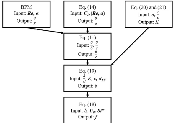
Figure 2 presents the process of PVS frequency estimation, indicating the independent input parameters with bold letters. The determination of K along with Eq. (20) and (21) will be discussed later.
Figure 2. Flowchart presenting the process of PVS frequency estimation. The independent input parameters are in bold.
6 SUPPLEMENTARY STUDY
The PVS studies reported in the literature are related predominantly to symmetrical blade profiles.
The literature studies have been supplemented and documented by the authors herein with a single case study, demonstrating the PVS phenomenon on a non-symmetrical blade profile. Further systematic case studies on PVS from non-symmetrical profiles are ongoing, and are planned to be reported in future publications. The case study presented herein was part of the MSc thesis work by E. Balla (Balla, 2015), under the supervision of Professor Alessandro Corsini at the Department of Mechanical and Aerospace Engineering, Faculty of Civil and Industrial Engineering, La Sapienza University.
The experimental layout on the RAF-6E profile documented in Balla and Vad, 2019, has been modelled using Computational Fluid Dynamics (CFD). The RAF-6E profile has been considered as being representative for a low-speed axial fan blade. The chord of the profile was c = 0.1 m and t/c
=0.1. The angle of attack was α = 13°. α = 13° is assigned nearly to the maximum lift coefficient, and is therefore representative for the operation of a fan blade of fully utilized loading capability. The Reynolds number is set to Re = 150 000, being a threshold for moderating the blade loss as recommended by Carolus, 2003. A structured mesh was created in Pointwise 17.2 R2. The mesh in the vicinity of the profile is shown in Figure 3. The bone shaped inner mesh was connected to a rectangular, block structured domain. The size of the computational domain was 1.5 meter in the streamwise, 0.15 meter in the spanwise and 1 meter in the cross-stream direction. These values are in accordance with the measurement setup reported in Balla and Vad, 2019. At the inlet a constant velocity profile was defined (U0 = 22 m/s), at the outlet zeroGradient was prescribed for every variable. All other boundaries were set as walls. The LES model, oneEqEddy was applied, along with the pisoFoam transient solver. The timestep was chosen to be 10-6 s in order to keep the Courant number below 1. The blade lift and drag coefficients were monitored during the simulation.
Figure 3. The mesh around the RAF6-E airfoil
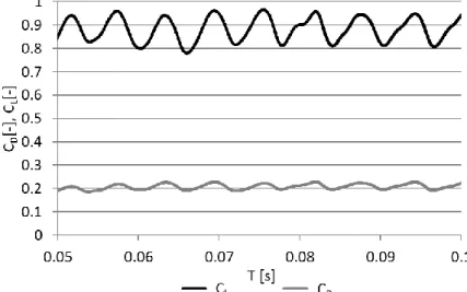
The effect of PVS is demonstrated herein using the temporarily fluctuating lift and drag coefficients as quantitative indicators, which are shown in Figure 4. The fluctuation of aerodynamic blade forces due to PVS are in the order of magnitude of ± 10 percent of the temporal mean lift and drag coefficient values. This draws the attention to the fact that PVS may be of significance not only from noise generation but also from mechanical vibration point of view. As the details of the unsteady velocity field indicate, the transversal distance between the shed vortex rows, b can be approximated as b ≈ c∙sinα in this particular case study. Therefore, b has been taken as 22 mm. The frequency of PVS, readable from Figure 4, is f = 160 Hz. Based on Eq. (18), the PVS Strouhal number St* is calculated as St* = fb/U0 = 160x0.022/22 = 0.16. Therefore, the case study supports that the universal
7
Strouhal number of St* = 0.16 (Yarusevych and Boutilier, 2011) can be assumed also for a non- symmetrical blade profile. The confirmation or refinement of this assumption via further systematic case studies on various non-symmetrical profiles is subject of future research.
Figure 4. The lift and drag coefficients as a function of time DETERMINATION OF MODEL PARAMETERS
A wide range of airfoil geometries and flow conditions has been included in the investigation.
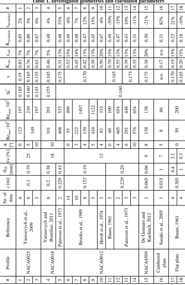
Their parameters are summarized in Table 1. On the right of the table, separated with a doubled line, are those parameters, which were determined by the authors.
In Table 1, the first and the last columns indicate the serial number of literature case under discussion. Cases will be referred to using these numbers from now on. In the ”Profile” column the types of the profiles are specified. In the next column the references are listed from which the data were obtained. The column labelled as ”Nr. of data” indicates the number of case studies incorporated in the given reference, and processed by the authors for obtaining Kcalc and s. In the next columns, the geometric parameters of the profiles: the chord length c, the trailing edge thickness dTE, and the maximum relative thickness t/c, are summarized. The flow conditions are presented in the forthcoming columns: the angle of attack α, and the minimum (Remin) and the maximum (Remax) of the investigated Reynolds number range corresponding to each case. In the column titled “St*” the values for the universal Strouhal number defined in Eq. (19) are listed. Case-specific St* values were possible to be calculated only for the measurements of Yarusevych et al., 2009, and Yarusevych and Boutilier, 2011, for which b data were directly obtained from the flow measurement results. For the other investigated cases its value was set to 0.16, based on Yarusevych and Boutilier, 2011. The data in the St* column indicate that the data vary about the mean value of St* = 0.16, within a relatively narrow range, thus demonstrating the reasonability of using St* = 0.16 as a universal value (Yarusevych and Boutilier, 2011). Among the parameters, which were determined by the authors, there is the Kcalc factor, which was calculated from the literature data. The uncertainty of Kcalc,which is denoted by εcalc, was estimated by the authors based on the setups and measurement conditions described in the literature. For each paper the parameters f, b, and U0 were gathered along with their uncertainty, if it was available. If the uncertainty of a parameter was not stated in the paper, its value would be estimated. An uncertainty propagation calculation was carried out to determine εcalc for each case. As f and b both depend on the frequency measurement uncertainty, they are not independent variables and thus as a pessimistic approach the overall uncertainty was calculated by summing the relative uncertainties of f, b, and U0. Kmodelled is determined with the new parametrization of K, discussed later on. εmodelled is the relative discrepancy of Kmodelled compared to Kcalc.
For most cases, data for more than one Reynolds number were available. Instead of listing all investigated values, the Reynolds number range is specified in Table 1. The investigated Reynolds number range depends on the geometry, as the profile geometry affects the value of the limiting Reynolds number (Relimit), above which the flow reattaches to the suction surface, and PVS can occur
8
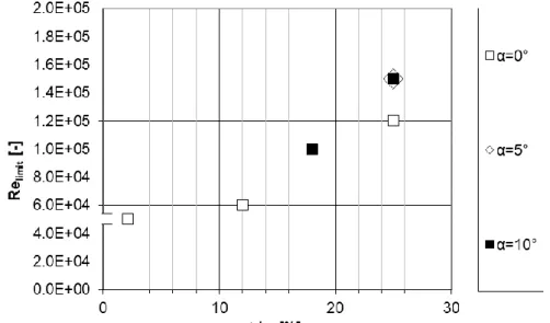
for an unstalled blade condition. Relimit values are shown as a function of t/c for various angles of attack in Figure 5. From the figure it can be seen that Relimit tends to increase with increasing t/c and α. With the increase of t/c and α, the suction side boundary layer thickens, and consequently, higher Reynolds number is needed for energizing the separated boundary layer in order to promote reattachment (Yarusevych and Boutilier, 2011). In Figure 5, cases #1, 2, 3, 4, 6, 17, and 18 are presented, as these cases included investigations on a wide Reynolds number range extending also to lower values, enabling the determination of Relimit. Below Relimit PVS does not occur, and thus makes the investigation at these low Reynolds numbers unnecessary.
Figure 5. The limiting Reynolds number as a function of relative thickness for various angles of attack
Based on the data in Table 1, and the Reynolds numbers corresponding to each case, θ/c and δ/c (from the BPM model) and CD could be calculated. For the NACA airfoils, CD was determined based on Sheldahl and Klimas, 1981, while for the flat plates it was computed from the Blasius drag law (Schlichting and Gersten, 2016). As no case-specific CD data was available for the cambered plate (Sasaki et al., 2005), the use of CD was omitted in that case.
In order to determine K, f as input data was required, which was available from the literature. A Reynolds number independent value of K was determined for each case in Table 1, as in the investigated range the effect of Reynolds number variance was negligible. Using K and St*, the value of s could also be calculated.
The semi-empirical model has iteratively been set providing best fitting to the literature data points.
Data related to α=0° have either been directly taken from the measurements or have been extrapolated from data related to nonzero angles of attack, self-consistently with the presented semi-empirical model. Using data corresponding to α=0°, K was determined in the function of relative thickness t/c [%], to provide best fitting. The calculated points and the fitted curve are shown in Figure 6. Case
#16 has been omitted from Figure 6, as it can be considered as an out-of-trend observation, as will be discussed later on. The size of the error bars are corresponding to the measurement uncertainties reported in Table 1. There is a good agreement between the modelled points and the fitting, with determination coefficient, R2 = 0.99. The value of K at α=0°can be determined with the use of the following polynomial
𝐾𝛼=0 = 1.7 ∙ 10−1+ 2.7 ∙ 10−2(𝑡
𝑐) (20)
where t/c is in percent. The fitted curve does not intersect the origin, it is shifted by a value of 0.16 in the positive direction. This suggests that even the boundary layers developing over the two surfaces of an infinitely thin flat plate at zero incidence, and interacting past the trailing edge, may exhibit a vortex street. This finding is confirmed by the works of Chase, 1972, and Voke and Potamitis, 1994.
As Figure 6 indicates, the value of K increases monotonically as t/c is increased.
9
Table 1. Investigated geometries and calculated parameters
The dependence on α [°] was determined for each t/c value separately. A second order polynomial was fitted to the data corresponding to each t/c. For all investigated t/c, the best fit could be achieved when the coefficient of the second order term is approximately -0.0019. Thus, the overall value of K can be calculated with the use of the following expression
# 1 2 3 4 5 6 7 8 9 10 11 12 13 14 15 16 17 18
εmodelled 2% 5% 6% 4% 55% -6% 7% 12% 15% -6% -30% -15% 10% -11% -21% 82% 21% -10%
Kmodelled 0.85 0.80 0.67 0.48 0.48 0.49 0.48 0.47 0.45 0.47 0.49 0.47 0.43 0.31 0.30 0.31 0.23 0.18
εcalc 7% 7% 7% 5% 13% 15% 14% 13% 13% 20% 15% 13% 13% 13% 20% n/a 15% 15%
Kcalc 0.83 0.76 0.63 0.46 0.31 0.52 0.45 0.42 0.39 0.50 0.70 0.55 0.39 0.35 0.38 0.17 0.19 0.20
s 0.19 0.165 0.155 0.165 0.175 0.175 n/a 0.170 0.165
St* 0.185 0.160 0.145 0.155
Remax/103 197 210 197 201 533 499 1122 333 100 654 448 654 138 86
Remin/103 123 101 468 55 222 139 416 83 60 465 291 576 138 8
α [°] 0 5 10 0 3 4 5 4 0 4 6 10 8 5
t/c [%] 9 7 2.1 0.3
dTE [mm] 0.38 0.43 0.06 1 6.4 1
c [m] 0.2 0.229 0.065 0.015
Nr. of data 4 6 3 6 2 14 10 8 5 3 3 2 3 3 1 1 4 4
Reference Yarusevych and Boutilier, 2011 Paterson et al., 1973 Hersh et al., 1974 Bauer, 1961 De Gennaro and Kuehnelt, 2012 Sasaki et al., 2005
Profile NACA4509 Cambered plate
# 1 2 3 4 5 6 7 8 9 10 11 12 13 14 15 16 17 180
0.160
1497 200
0.170 0.165 0.175
149 50Bauer, 1961Flat plate
NACA0025 0.305
0.290.229
10
25 18 12
0.79 0.19Brooks et al., 1989 Paterson et al., 1973
NACA0018 NACA0012
0.3 0.152
Yarusevych et al., 2009
10
𝐾 = 𝐾𝛼=0− 1.8 ∙ 10−3𝛼2 (21)
for which Kα=0 is to be taken from Eq. (20).
Figure 6. The value of K as a function of relative thickness
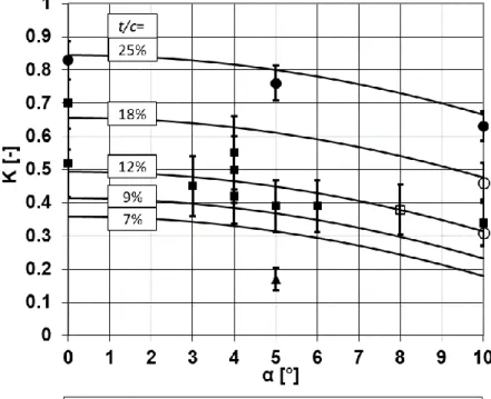
The fitted curves, along with the measurement points are presented in Figure 7. The size of the error bars correspond to the highest uncertainties reported in Table 1 for each t/c. Those cases for which a single measurement point, related to α = 0, was only available, are excluded from Figure 7.
In all investigated cases, the value of K decreases as α increases. For airfoils of different t/c the fitted curves have the same shape and there is only a constant shift as a result of change in relative thickness.
Most of measurement-based points fit the model curve within measurement uncertainty. The highest discrepancy, occurring for the blade of t/c = 7% (Sasaki et al., 2005) can be explained by the fact that in Sasaki et al., 2005, measurements were made on a fan blading with high solidity, while the universal Strouhal number concept and the BPM model were elaborated for isolated airfoils.
Figure 7. The value of K as a function of angle of attack for different relative thicknesses.
Solid lines indicate the modelled curve for each relative thickness, and the markers indicate the measurement points
After the value of K was determined for each case, s was also calculated. The calculated values are summarized in Table 1. For the investigated cases, s was always below the theoretical value of
11
0.281. Based on the calculated data, the new proposed empirical value is s = 0.17, which is the average of s values for all cases investigated.
UNCERTAINTY ANALYSIS
In order to estimate the overall uncertainty of the empirical model formulated in Eq. (20) and (21), the value of K for each case was determined with Eq. (21) (Kmodelled) and compared to the values calculated from measurement data (Kcalc). The values of K along with the relative discrepancy, εmodelled
are shown in Table 1. There are two remarkably high discrepancy values (#5 and #16). The discrepancies of these two cases are more than 1.5 times higher than the next highest one (#11, 25%).
These data can be considered as out-of-trend observations and were arbitrarily excluded from the overall uncertainty estimation of the model. Without the aforementioned two cases, the average relative discrepancy is 11%. Even for cases #5 and #16, the present model still performs better compared to using previous approximation of K ≈0.5-0.6 (Hersh et al., 1974, Fathy et al., 1977, Lee et al., 1993, Dou et al., 2016). The discrepancy from the present model in case #16 can be explained, as already mentioned, with the high solidity of the fan blading. Compared to K =0.5 (Fathy et al., 1977), the elaborated empirical model performs as good or even better in all cases, while compared to K =0.6 (Hersh et al., 1974, Lee et al., 1993, Dou et al., 2016), the model is outperformed in case
#11 only.
CONCLUSION AND FUTURE REMARKS
Based on literature data, an empirical formula for factor K has been determined as a function of relative thickness and angle of attack. With the use of K, vortex shedding frequencies for various profile geometries can be determined. The polynomials, which were proposed in Eq. (20) and (21), can be easily implemented in engineering applications. The following trends were observed:
The value of K increases as t/c increases at α = 0.
The value of K decreases as α increases.
A new value, s=0.17, was proposed for flows past realistic airfoils, in spite of s = 0.281 used in Hersh et al., 1974, Fathy et al., 1977, Lee et al., 1993 and Dou et al., 2016.
The average uncertainty of the model is 11%, however, it still outperforms the approximation which was used until now. The model could be further refined with detailed aerodynamic and aeroacoustic data on non-symmetric profiles, with various relative cambers.
ACKNOWLEDGEMENTS
This work has been supported by the Hungarian National Research, Development and Innovation Centre under contract No. K 119943 and by the ÚNKP-18-3-I New National Excellence Program of the Hungarian Ministry of Human Capacities. The research reported in this paper was supported by the Higher Education Excellence Program of the Ministry of Human Capacities in the frame of Water science & Disaster Prevention research area of Budapest University of Technology and Economics (BME FIKP-VÍZ).
Gratitude is expressed to Professor Alessandro Corsini for supervising the MSc thesis of Ms. Balla, and to Dr. Giovanni Delibra for his valuable advice on the thesis.
REFERENCES
Balla, E., Aerodynamic and aeroacoustic behaviour of airfoils, MSc Thesis, Budapest University of Techology and Economics (2015)
Balla, E., Vad, J., Lift and drag force measurements on basic models of low-speed axial fan blade sections, Proceedings of the Institution of Mechanical Engineers, Part A: Journal of Power and Energy, 233(2) (2019) 165-175.
Bauer, A. B., Vortex shedding from thin flat plates parallel to the free stream, Journal of the Aerospace Sciences, 28(4) (1961) 340-341.
Bearman, P. W., On vortex street wakes. Journal of Fluid Mechanics, 28(4) (1967) 625-641.
12
Borges SS., CFD techniques applied to axial fans design of electric motors, In: Proceedings of the international conference on fan noise, technology and numerical methods (FAN2012), Senlis, France.
Brooks, T. F., Marcolini, M. A., Scaling of airfoil self-noise using measured flow parameters. AIAA Journal, 23(2), (1985) 207-213.
Brooks, T. F., Pope, D. S., Marcolini, M. A., Airfoil self-noise and prediction, NASA Reference Publication NASA-RP-1219. 1989
Carolus T. Ventilatoren. Wiesbaden: B. G. Teubner Verlag, 2003.
Chase, D. M. Sound radiated by turbulent flow off a rigid half‐plane as obtained from a wavevector spectrum of hydrodynamic pressure. The Journal of the Acoustical Society of America, 52(3B), (1972) 1011-1023.
De Gennaro, M., Kuehnelt, H., Broadband noise modelling and prediction for axial fans, In Proceedings of the International Conference Fan Noise, Technology and Numerical Methods, Paris, France (2012).
Dou, H., Li, Z., Lin, P., Wei, Y., Chen, Y., Cao, W., He, H., An improved prediction model of vortex shedding noise from blades of fans, Journal of Thermal Science, 25(6) (2016) 526-531.
Fathy, A., Rashed, M. I., Lumsdaine, E., A theoretical investigation of laminar wakes behind airfoils and the resulting noise pattern, Journal of Sound and Vibration, 50(1) (1977) 133-144.
Fink, M. R. Prediction of airfoil tone frequencies. Journal of Aircraft, 12(2), (1975) 118-120.
Gue, F, Cheong, C, Kim, T., Development of low-noise axial cooling fans in a household refrigerator, J Mech Sci Technol, 25 (2011) 2995–3004.
Hersh, A. S., Sodermant, P. T., Hayden, R. E., Investigation of acoustic effects of leading-edge serrations on airfoils, Journal of Aircraft, 11(4) (1974) 197-202.
Hooker, S. G. On the action of viscosity in increasing the spacing ratio of a vortex street. Proc. R.
Soc. Lond. A, 154(881) (1936) 67-89
Huang, LX., Characterizing computer cooling fan noise, J Acoust Soc Am, 114 (2003) 3189–3200 Migliore, P., Oerlemans, S., Wind tunnel aeroacoustic tests of six airfoils for use on small wind turbines, Journal of Solar Energy Engineering, 126(4) (2004), 974-985
Lee, C:, Chung, M. K., Kim, Y. H., A prediction model for the vortex shedding noise from the wake of an airfoil or axial flow fan blades, Journal of Sound and Vibration. 164 (2) (1993) 327-336 Paterson, R. W., Vogt, P. G., Fink, M. R.,Munch, C. L., Vortex noise of isolated airfoils, Journal of Aircraft, 10(5) (1973) 296-302.
Sasaki, S., Kodama, Y., Hayashi, H., Hatakeyama, M., Influence of the Karman vortex street on the broadband noise generated from a multiblade fan, Journal of Thermal Science, 14(3) (2005) 198-205.
Schlichting, H., Gersten, K. Boundary-layer theory. Springer. (2016).
Sheldahl, R. E., Klimas, P. C., Aerodynamic characteristics of seven symmetrical airfoil sections through 180-degree angle of attack for use in aerodynamic analysis of vertical axis wind turbines (No.
SAND-80-2114). Sandia National Labs., Albuquerque, NM (USA) (1981)
Vad, J, Horváth, Cs, Kovács, JG., Aerodynamic and aero-acoustic improvement of electric motor cooling equipment, Proc IMechE, Part A: J Power and Energy, 228 (2014) 300–316.
Voke, P. R., Potamitis, S. G.. Numerical simulation of a low‐Reynolds‐number turbulent wake behind a flat plate. International Journal for Numerical Methods in Fluids, 19(5), (1994), 377-393.
Yarusevych, S., Sullivan, P. E., Kawall, J. G. On vortex shedding from an airfoil in low-Reynolds- number flows, Journal of Fluid Mechanics. 632 (2009) 245-271.
Yarusevych, S., H. Boutilier, M. S., Vortex shedding of an airfoil at low Reynolds numbers, AIAA Journal, 49(10) (2011) 2221-2227