Annales Mathematicae et Informaticae (34.)

ANNALES MATHEMATICAE ET INFORMATICAE 34. (2007)

HUNGARIA, EGER

ES

ZTERHÁZYKÁROLY CO

LL EGE

EGER 1774

COMMISSIO REDACTORIUM

Sándor Bácsó (Debrecen), Sonja Gorjanc (Zagreb), Tibor Gyimóthy (Szeged), Miklós Hoffmann (Eger), József Holovács (Eger), László Kozma (Budapest), Kálmán Liptai (Eger), Florian Luca (Mexico), Giuseppe Mastroianni (Potenza), Ferenc Mátyás (Eger), Ákos Pintér (Debrecen), Miklós Rontó (Miskolc, Eger),

János Sztrik (Debrecen, Eger), Gary Walsh (Ottawa)



TOMUS 34. (2007)

ANNALES

MATHEMATICAE ET

INFORMATICAE

ANNALES

MATHEMATICAE ET INFORMATICAE

VOLUME 34. (2007)

EDITORIAL BOARD

Sándor Bácsó (Debrecen), Sonja Gorjanc (Zagreb), Tibor Gyimóthy (Szeged), Miklós Hoffmann (Eger), József Holovács (Eger), László Kozma (Budapest), Kálmán Liptai (Eger), Florian Luca (Mexico), Giuseppe Mastroianni (Potenza), Ferenc Mátyás (Eger), Ákos Pintér (Debrecen), Miklós Rontó (Miskolc, Eger),

János Sztrik (Debrecen, Eger), Gary Walsh (Ottawa)

INSTITUTE OF MATHEMATICS AND COMPUTER SCIENCE ESZTERHÁZY KÁROLY COLLEGE

HUNGARY, EGER

HU ISSN 1787-5021 (Print) HU ISSN 1787-6117 (Online)

A kiadásért felelős:

az Eszterházy Károly Főiskola rektora Megjelent az EKF Líceum Kiadó gondozásában

Kiadóvezető: Kis-Tóth Lajos Felelős szerkesztő: Zimányi Árpád Műszaki szerkesztő: Tómács Tibor Megjelent: 2007. december Példányszám: 50

Készítette: Diamond Digitális Nyomda, Eger Ügyvezető: Hangácsi József

Annales Mathematicae et Informaticae 34(2007) pp. 3–8

http://www.ektf.hu/tanszek/matematika/ami

A modification of Graham’s algorithm for determining the convex hull of a finite

planar set

Phan Thanh An

Institute of Mathematics

Vietnamese Academy of Science and Technology e-mail: thanhan@math.ac.vn

Submitted 4 September 2007; Accepted 11 October 2007

Abstract

In this paper, in our modification of Graham scan for determining the convex hull of a finite planar set, we show a restricted area of the examination of points and its advantage. The actual run times of our scan and Graham scan on the set of random points shows that our modified algorithm runs significantly faster than Graham’s one.

Keywords: Algorithm, computational complexity, convex hull, extreme point, Graham scan

MSC:52B55, 52C45, 65D18

1. Introduction

The determination of the convex hull of a point set has successfully been applied in application domains such as pattern recognition [2], data mining [3], stock cutting and allocation [4], or image processing [10].

Graham’s algorithm [5] is an important sequential algorithm used for determin- ing the convex hull of the set of n points in the plane (n > 3). This algorithm has a complexity of O(nlogn). Take an interior point x of the convex hull and assume without loss of generality that no three points of the given set (including x) are collinear. We will use the phrase “convex hull” to mean “the set of extreme points of the convex hull”. The first step of Graham’s algorithm is to construct a sequence P = {p1, . . . , pn} of the points in polar coordinates ordered about x in terms of increasing angle (see Fig. 1) (note that pointp1is adjacent topn). In this sequence, call a pointreflexif the interior angle made by it and its adjacent points

3

4 P.T. An is greater thanπ. In Fig. 1, p1 is nonreflex andp2 is reflex. Then, a reflex point does not belong to the convex hull. Graham scan in the algorithm examines the points of the sequence in counterclockwise order and deletes those that are reflex;

upon termination, only nonreflex points remain, so the rest is the convex hull ofP. Several modifications of Graham’s algorithm have been proposed, all having to do with the following. If the first point inP is guaranteed to be on the convex hull, then it is never reflex (see [1, 6, 9, 10, 11] etc).

p p

x

p p

p

p 1

2 3 i

i−1

Figure 1: The first step of Graham’s algorithm constructs a se- quenceP={p1, . . . , pn}of the points in polar coordinates ordered

aboutx.

Determining when the counterclockwise examination of points can stop seems to be the major difficulty, because deleting a reflax point can change its neighbors from nonreflex to reflex. That is one of the reasons why some of modifications of Graham’s algorithm contain errors (see [7]). In this note, in our modification of Graham scan, we show a restricted area of the examination of points and its advantage. The actual run times of our scan and Graham scan on the set of random points are given in Table 1, which shows that our modified algorithm runs significantly faster than Graham’s one.

2. A modification of the Graham scan

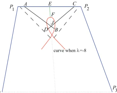
We shall shortly describe a restricted area of the examination of points in Gra- ham scan. Suppose that αis some compact convex set containingP (see Fig. 2).

The first step of Graham’s algorithm constructs a sequenceP ={p1, . . . , pn}of the points in polar coordinates ordered about the interior pointxin terms of increasing angle. After that, let pi−1 be nonreflex (i.e., the interior angle made by it and pi

and pi−2 is less thanπ). Let the raysxpi andpi−1pi intersect the boundary ofα atui andvi, respectively (see Fig. 2). Denoteu[ixvi and[u[ixvi]the angle at point xand the area, respectively, formed by raysxui andxvi.

A modification of Graham’s algorithm . . . 5

x 1

p

v u

p=q p=q

i i−1 l

1

pn

v’_i

i i

β u’_i

α

Figure 2: αcontainsPand the restricted area at pointpiis[u[ixvi].

Ifα⊂βthen[u[ixvi]⊂[u[^′_ixv_i^′].

Proposition 2.1. Let the rays xpi and pi−1pi intersect the boundary of α at ui

andvi, respectively. Ifpi−1 is nonrelfex and all points ofP ∩[u[ixvi]are nonreflex, thenpi is nonrelfex, too.

Proof. Assume thatpi+1, . . . , pk∈[u[ixvi] andpj∈/[u[ixvi]fork+16j6n. Since α is convex, the intersection of α and the closed half-plane bounded by the line pi−1pi and containingxis convex. It follows that pi−1\pipj < πfork+ 16j6n.

Therefore,pi−1\pipj < πfori+ 16j6n. Since pi−1 is nonreflex,pi is nonreflex,

too.

By Proposition 2.1, to examine ifpiis nonreflex or not, we only need to examine if pi is nonreflex or not with the points ofP in counterclockwise order beginning frompi+1and belonging to[u[ixvi]. We now present our modification for Graham’s algorithm.

Algorithm:

First, find interior pointx; label itp0. Then sort all other points angularly about x; labelp1, . . . , pn. SetP ={p1, . . . , pn}. Take a compact convex setαcontaining these points. We now determine the convex hullQ={q1, . . . , ql+1}.

1. Begin at p1. Set l = 1and i= 2. Becausep1 is on the convex hull, we have q1=p1.

2. Consider ql. If i = n, go to 3. Else, let the rays xql and qlpi intersect the boundary ofαat ui andvi, respectively.

6 P.T. An 2.1Setm= 1.

2.2 If pi\xpi+m 6 p[ixvi (i.e., pi+m ∈ P ∩[u[ixvi]) and ql\pipi+m < π, then set m=m+ 1and go to 2.2. Else either

\

pixpi+m > p[ixvi, then by Proposition 2.1, pi is nonreflex, set ql+1 = pi, i=i+ 1andl=l+ 1 go to2, or

ql\pipi+m> π, thenq\lpipk < π for allpk∈ P, i < k < i+m. Set i=i+m, go to2.

3. Setql+1=pn. Then,Q={q1, . . . , ql+1}is the convex hull. STOP.

Note thatxcan be chosen to be a point on the convex hull (see [1, 9]).

Proposition 2.2. The algorithm computes the convex hull in n(logn)time.

Proof. By Proposition 2.1, points ofQare nonreflex. Hence, the algorithm com- putes the convex hull.

After sorting points that requires n(logn) time, the algorithm can only take linear time, since it only advances, never backs up, and the number of steps is therefore limited by the number of points of P. Therefore, the algorithm runs in

n(logn)time.

Proposition 2.3. Suppose that α and β are compact convex sets containing P. Let the rays xpi andpi−1pi intersect the boundary ofα(β, respectively) at ui and vi (atu^′_i andv_i^′, respectively). Ifα⊂β then[u[ixvi]⊂[u[^′_ixv_i^′].

Proof. Since α, β are convex and α ⊂ β, vi belongs to the segment [v_i^′, pi]. It

follows that [u[ixvi]⊂[u[^′_ixv_i^′].

Our modification only need to examine the points of P in counterclockwise order beginning from pi and belonging to [u[ixvi] while Jarvis’s algorithm [8] and variations of Graham’s convex hull algorithm like Akl-Toussaint’s algorithm [1], Graham-Yao’s algorithm [6], Toussaint-Avis’s algorithm [11], etc require that for many points. By Proposition 2.3, the execution time is reduced if the set α is enough small such that it still contains P. So we can choose αto be the smallest rectangleU enclosingP and having sides parallel to the coordinate lines.

The algorithm requires to check the conditionpi\xpi+m6p[ixvi. This is imple- mented in our code as follows: Let xpi+mintersectuivi atp¯i+m. Thenpi\xpi+m6

[

pixvi iffx-coordinate ofp¯i+m is betweenx-coordinates ofui andvi.

For a given setPof points randomly positioned in some rectangleVhaving sides parallel to the coordinate lines, we can take this rectangle to be α. Based on the

“throw-away” principle [1], we can assume thatP includes a finite number of points randomly positioned in the interior of the right-angled triangle abc having sides parallel to the coordinate lines and two pointsbandc (which form the hypotenuse of the triangle).

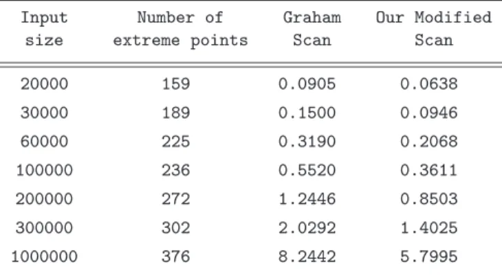
A modification of Graham’s algorithm . . . 7 Our modified algorithm is implemented in C code. To compare it with Graham’s algorithm we use an implementation of Graham’s algorithm written by O’Rourke [9]. Codes are compiled by the GNU C Compiler under SuSe Linux 10.0 and are executed on a Pentium IV processor. For the comparison to be meaningful, both implementations use the same code for file reading and rotary sort. The actual run times of the scans in our algorithm and Graham’s algorithm on such setP are given in Table 1, which shows that our modified algorithm runs significantly faster than Graham’s one (with integer coordinates). In this case, α=U =V.

Input Number of Graham Our Modified size extreme points Scan Scan

20000 159 0.0905 0.0638

30000 189 0.1500 0.0946

60000 225 0.3190 0.2068

100000 236 0.5520 0.3611

200000 272 1.2446 0.8503

300000 302 2.0292 1.4025

1000000 376 8.2442 5.7995

Table 1: The actual run times of scans in our algorithm and Gra- ham’s algorithm (time in sec) on a finite number of points randomly positioned in the interior of the right-angled triangle abc of size 40000 having sides parallel to the coordinate lines and two points

bandc.

References

[1] Akl, S.G.and Toussaint, G.T., A fast convex hull algorithm,Information Pro- cessing Letters, 7 (1978) 219–222.

[2] Akl, S.G.andToussaint, G.T., Efficient convex hull algorithms for pattern recog- nition applications,Int. Joint Conf. on Pattern Recognition, Kyoto, Japan, (1978) 483–487.

[3] Böhm, C.and Kriegel, H., Determing the convex hull in large multidimensional databases,Proceedings of the Third International Conference on Data Warehousing and Knowledge Discovery, Lecture Notes in Computer Science, Springer-Verlag,2114 (2001) 294–306.

[4] Freeman, H.andShapira, R., Determining the minimum-area encasing rectangle for an arbitrary closed curve,Comm. ACM, 18(7) (1975).

8 P.T. An [5] Graham, R.L., An efficient algorithm for determining the convex hull of a finite

planar set,Information Processing Letters, 26 (1972) 132–133.

[6] Graham, R.L.andYao, F.F., Finding the convex hull of a simple polygon,Journal of Algorithms, 4 (1983) 324–331.

[7] Gries, D.and Stojmenovic’, I., A note on Graham’s convex hull algorithm, In- formation Processing Letters, 25 (1987) 323–327.

[8] Jarvis, R.A., On the identication of the convex hull of a finite set of points in the plane,Information Processing Letters, 2 (1973) 18–21.

[9] O’Rourke, J., Computational Geometry in C,Cambridge University Press, Second Edition, 1998.

[10] Rosenfeld, A., Picture Processing by Computers, Academic Press, New York, 1969.

[11] Toussaint, G.T. and Avis, D., On convex hull algorithm for polygons and its application to triangulation problems,Pattern Recognition, 15, No. 1 (1982) 23–29.

Phan Thanh An Institute of Mathematics

Vietnamese Academy of Science and Technology 18 Hoang Quoc Viet Road, 10307 Hanoi, Vietnam

Annales Mathematicae et Informaticae 34(2007) pp. 9–16

http://www.ektf.hu/tanszek/matematika/ami

Remarks on the Lie derived lengths of group algebras of groups with cyclic

derived subgroup

Zsolt Balogh

, Tibor Juhász

aInstitute of Mathematics and Informatics, College of Nyíregyháza e-mail: baloghzs@nyf.hu

bInstitute of Mathematics and Informatics, Eszterházy Károly College e-mail: juhaszti@ektf.hu

Submitted 20 June 2007; Accepted 10 November 2007

In memoriam Professor Péter Kiss Abstract

The aim of this paper is to give a new elementary proof for our previous theorem, in which the Lie derived length and the strong Lie derived length of group algebras are determined in the case when the derived subgroup of the basic group is cyclic of odd order.

Keywords: Group algebras, Lie derived length MSC:16S34, 17B30

1. Introduction

The group algebraF G of a groupGover a fieldF may be considered as a Lie algebra with the usual bracket operation [x, y] = xy−yx. Denote by [X, Y] the additive subgroup generated by all Lie products[x, y]withx∈X and y∈Y, and define the Lie derived series and the strong Lie derived series of the group algebra F G respectively, as follows: letδ^[0](F G) =δ⁽⁰⁾(F G) =F Gand

δ^[n+1](F G) =

δ^[n](F G), δ^[n](F G) , δ⁽ⁿ⁺¹⁾(F G) =

δ⁽ⁿ⁾(F G), δ⁽ⁿ⁾(F G) F G.

We say that F G is Lie solvable if δ^[m](F G) = 0 for some m and the number dlL(F G) = min{m∈ N | δ^[m](F G) = 0} is called the Lie derived length of F G.

9

10 Zs. Balogh, T. Juhász Similarly,F Gis said to be strongly Lie solvable of derived lengthdl^L(F G) =mif δ^(m)(F G) = 0 andδ^(m−1)(F G)6= 0. Evidently, δ^[i](F G)⊆δ⁽ⁱ⁾(F G)for alli.

Form>0let

s^(m)_l =







1 if l= 0;

2s^(m)_l−1+ 1 if s^(m)_l−1 is divisible by 2^m; 2s^(m)_l−1 otherwise.

In [1] we proved the following

Theorem 1.1 (Z. Balogh and T. Juhász [1]). LetGbe a group with cyclic derived subgroup of orderpⁿ, wherepis an odd prime, and letF be a field of characteristic p. IfG/CG(G^′)has order 2^mp^r, then

dlL(F G) = dl^L(F G) =d+ 1,

whered is the minimal integer for which s^(m)_d >pⁿ holds. Otherwise, dlL(F G) = dl^L(F G) =⌈log₂(2pⁿ)⌉.

This article can be considered as a supplement to [1]. In the original proof of the theorem, at the discussion of the cases when either G/CG(G^′)has order 2p^r, or the order of G/CG(G^′)is divisible by some odd prime q 6=p, Theorem A and B from [3] play the central role. Two lemmas are shown here, which enable us to construct a new (elementary) proof of Theorem 1.1 avoiding the use of above- mentioned results of A. Shalev. For a change, we prove these two lemmas by two different ways (the first was proposed by the referee, whereat we wish to thank him), although both statements could be proved by both methods which will be presented here.

We denote by ω(F G) the augmentation ideal of F G. It is well-known that ω(F G) is nilpotent if and only if G is a finite p-group and char(F) = p. The nilpotency index ofω(F G)will be denoted byt(G). For a normal subgroupH⊆G we mean by I(H) the ideal F G· ω(F H). For x, y ∈ G let x^y = y⁻¹xy and (x, y) =x⁻¹x^y, furthermore, denote by ζ(G)the center of the groupG. We shall use freely the identities

[x, yz] = [x, y]z+y[x, z], [xy, z] =x[y, z] + [x, z]y, and for units a, bthe equality[a, b] =ba (a, b)−1

.

2. Proof of Theorem 1.1

LetGbe a group with derived subgroupG^′=hx|x^pn = 1iwhere pis an odd prime, and let F be a field of characteristicp. As it is well-known, the automor- phism group of G^′ is isomorphic to the unit groupU(Zpⁿ) of Zpⁿ. Furthermore, U(Zpⁿ)is cyclic, so the factor groupG/CG(G^′), which is isomorphic to a subgroup of U(Zpⁿ), is cyclic, too. We distinguish the following two cases according to the order ofG/CG(G^′).

Remarks on the Lie derived lengths of group algebras . . . 11

2.1. G/C has order 2

p

Letdbe the minimal integer for whichs^(m)_d >pⁿ holds.

First suppose that m= 0. Then, as is easy to check (see [1]), the group Gis nilpotent, and by [2],dlL(F G) = dl^L(F G) =⌈log₂(pⁿ+ 1)⌉. Since

2^d−1 =s⁽⁰⁾_d−1< pⁿ 6s⁽⁰⁾_d = 2^d+1−1,

we haved <log₂(pⁿ+ 1)6⌈log₂(pⁿ+ 1)⌉6d+ 1, thus Theorem 1.1 is proved for the case in point.

Let now m > 1. To prove that d+ 1 is an upper bound on dl^L(F G) it is sufficient to show that

δ^(l+1)(F G)⊆I(G^′)^s(m)l for all l>0.

This is clear for l= 0. For the induction we need Lemma 2from [1], which states that

[I(G^′)^i2m,I(G^′)^j2m]⊆I(G^′)^i2m+j2m+1. (2.1) Hence, assuming thatδ^(l)(F G)⊆I(G^′)^s(m)l−1, we obtain

δ^(l+1)(F G) = [δ^(l)(F G), δ^(l)(F G)]F G

⊆[I(G^′)^s(m)l−1,I(G^′)^s(m)l−1]F G⊆I(G^′)^s(m)l .

Therefore, dl^L(F G)6d+ 1. Now, we shall prove thatd+ 16dlL(F G). Let us choose an element aCG(G^′) of order 2^m from G/CG(G^′) and consider the group H =hx, aiand setx^k =x^a. In particular, whenm= 1, we have thata²∈ζ(H), x^a=x⁻¹, and the quotient groupH=H/ζ(H)is isomorphic to the dihedral group of order2pⁿ. This case is treated in the next lemma.

Lemma 2.1. Let Gbe the dihedral group of order2pⁿ for some odd primep, and letchar(F) =p. Then dlL(F G)>d+ 1, wheredis the minimal integer such that s⁽¹⁾_d >pⁿ.

Proof. Write the groupGasha, x|a²=x^pn = 1, xa=ax⁻¹iand setsl=s⁽¹⁾_l . We shall show that(x−x⁻¹)^sl−1 ∈δ^[l](F G)iflis odd, and(x−x⁻¹)^sl−1+1∈δ^[l](F G) ifl is even; further

a(x−x⁻¹)^sl−1 ∈δ^[l](F G) and ax(x−x⁻¹)^sl−1 ∈δ^[l](F G).

For, ifl= 1 thenx−x⁻¹= [a, ax]∈δ^[1](F G),a(x−x⁻¹) = [a, x]∈δ^[1](F G) andax(x−x⁻¹) = [ax, x]∈δ^[1](F G).

Iflis even then, by induction, the elements

(x−x⁻¹)^sl−2 , a(x−x⁻¹)^sl−2, ax(x−x⁻¹)^sl−2

12 Zs. Balogh, T. Juhász belong toδ^[l−1](F G). Since(x−x⁻¹)² is central andsl−2 is odd,

[ax(x−x⁻¹)^sl−2, a(x−x⁻¹)^sl−2] = [ax(x−x⁻¹), a(x−x⁻¹)](x−x⁻¹)^2sl−2−2

=a(x−x⁻¹)[x, a(x−x⁻¹)](x−x⁻¹)^2sl−2−2

= (x−x⁻¹)^2sl−2+1= (x−x⁻¹)^sl−1+1. Thus(x−x⁻¹)^sl−1+1∈δ^[l](F G). Furthermore,

[1

2a(x−x⁻¹)^sl−2,(x−x⁻¹)^sl−2] = [1

2a,(x−x⁻¹)^sl−2](x−x⁻¹)^sl−2

= [1

2a, x−x⁻¹](x−x⁻¹)^2sl−2−1

=a(x−x⁻¹)^2sl−2 =a(x−x⁻¹)^sl−1, and hence,

[1

2ax(x−x⁻¹)^sl−2,(x−x⁻¹)^sl−2] = [1

2a(x−x⁻¹)^sl−2,(x−x⁻¹)^sl−2]x

=ax(x−x⁻¹)^sl−1,

so the elementsa(x−x⁻¹)^sl−1 andax(x−x⁻¹)^sl−1 belong toδ^[l](F G).

Now, iflis odd thensl−2 is even, and by the inductive hypothesis (x−x⁻¹)^sl−2+1, a(x−x⁻¹)^sl−2, ax(x−x⁻¹)^sl−2 ∈δ^[l−1](F G).

As above,

[a(x−x⁻¹)^sl−2, ax(x−x⁻¹)^sl−2] = [a, ax](x−x⁻¹)^2sl−2

= (x−x⁻¹)^2sl−2+1

= (x−x⁻¹)^sl−1 ∈δ^[l](F G), and

[1

2a(x−x⁻¹)^sl−2,(x−x⁻¹)^sl−2+1] = [1

2a, x−x⁻¹](x−x⁻¹)^2sl−2

=a(x−x⁻¹)^2sl−2+1

=a(x−x⁻¹)^sl−1∈δ^[l](F G), and finally

[1

2ax(x−x⁻¹)^sl−2,(x−x⁻¹)^sl−2+1] = [1

2a(x−x⁻¹)^sl−2,(x−x⁻¹)^sl−2+1]x

=ax(x−x⁻¹)^sl−1 ∈δ^[l](F G).

Induction is complete.

Letdbe the minimal integer such thatsd>pⁿ. Thensd−1< pⁿ and a(x−x⁻¹)^sd−1 =ax^−sd−1(x²−1)^sd−1

is nonzero element ofδ^[d](F G)(by the binomial theorem as the order ofx² ispⁿ).

ThusdlL(F G)> dand the statement follows.

Remarks on the Lie derived lengths of group algebras . . . 13 The following line shows the truth of Theorem 1.1 for the casem= 1:

d+ 16dlL(F H)6dlL(F H)6dlL(F G).

Let us turn to the casem >1. Since (x, a) =x^−1+k ∈H^′ andk6≡1 (modp), we have that H^′ has orderpⁿ. Moreover, H/CH(H^′)has order2^m. Lemma 4 in [1]

forces

aω^s(m)l (F H^′)⊕a⁻¹ω^s(m)l (F H^′)⊆δ^[l+1](F H)

for alll>0, thereforeδ^[d](F H)6= 0, so d+ 16dlL(F H)6dlL(F G), as asserted.

2.2. The order of G/C

(G

) is divisible by some odd prime q 6 = p

In the proof of the next lemma we will use the well-known congruence

x^k−1≡k(x−1) (mod I(G^′)²) for all k∈Z. (2.2) SetG/CG(G^′) =hbCG(G^′)iandx^k =x^b. The congruence

[(x−1)^2l, b]≡(k^2l−1)b(x−1)^2l (modI(G^′)^2l+1) for all l>0 (2.3) can be obtained as a simple consequence of (2.2).

Lemma 2.2. Let G be a group with cyclic derived subgroup of order pⁿ and let char(F) =p. If the order of G/CG(G^′) is divisible by an odd prime q 6=p, then dlL(F G)>⌈log₂(2pⁿ)⌉.

Proof. Let G^′ = hx | x^pn = 1i and let us choose an element bC ∈ G/CG(G^′) of order q and set x^k = x^b. Evidently, k^2m 6≡ 1 (modp) for all m. Set H = hb, CG(G^′)i. Clearly, x^k−1 = (x, b)∈ H^′ is of order pⁿ, so H^′ has order pⁿ, too.

SinceH^′ = (b, CG(G^′))and the mapc7→(b, c)is an epimorphism of CG(G^′)onto H^′, we can choose c fromCG(G^′)such that(b, c) =x. Define the following three series in F G: let

u0=b, v0=c, w0=c⁻¹b⁻¹, and, forl>0, let

ul+1= [ul, vl], vl+1= [ul, wl], wl+1= [wl, vl].

Using induction we show for oddl that

ul≡t^(l)_u cb(x−1)^2l−1 (mod I(G^′)^2l−1+1);

vl≡t^(l)_v c⁻¹(x−1)^2l−1 (modI(G^′)^2l−1+1);

wl≡t^(l)_wb⁻¹(x−1)^2l−1 (modI(G^′)^2l−1+1),

(2.4)

14 Zs. Balogh, T. Juhász and ifl is even then

ul≡t^(l)_u b(x−1)^2l−1 (modI(G^′)^2l−1+1);

vl≡t^(l)_v c(x−1)^2l−1 (modI(G^′)^2l−1+1);

wl≡t^(l)_wc⁻¹b⁻¹(x−1)^2l−1 (modI(G^′)^2l−1+1),

(2.5)

where t^(l)u , t^(l)v , t^(l)w are nonzero elements in the field F while2^l−1< pⁿ. Evidently, u1= [b, c] =cb(x−1), and applying (2.2) we have

v1= [b, c⁻¹b⁻¹] =c⁻¹ (x⁻¹)^b−1−1

=c⁻¹(x^−k′ −1)≡ −k^′c⁻¹(x−1) (modI(G^′)²),

and similarly,w1 = [c⁻¹b⁻¹, c] ≡ −k^′b⁻¹(x−1) (modI(G^′)²), wherex^k′ =x^b−1. Therefore (2.4) holds for l = 1. Now assume that (2.4) is true for some odd l.

Then, using the congruences (2.3) andkk^′≡1 (modp), we have ul+1≡t^(l)_u t^(l)_v [cb(x−1)^2l−1, c⁻¹(x−1)^2l−1]

≡ −t^(l)_u t^(l)_v [(x−1)^2l−1, b](x−1)^2l−1

≡ −t^(l)_u t^(l)_v (k^2l−1−1)b(x−1)^2l (modI(G^′)^2l+1), vl+1≡t^(l)_u t^(l)_w[cb(x−1)^2l−1, b⁻¹(x−1)^2l−1]

≡t^(l)_u t^(l)_w −b⁻¹c[(x−1)^2l−1, b](x−1)^2l−1 +cb[(x−1)^2l−1, b⁻¹](x−1)^2l−1

≡t^(l)_u t^(l)_wk^2l−1(k^′2l−1)c(x−1)^2l (modI(G^′)^2l+1) and

wl+1≡t^(l)_wt^(l)_v [b⁻¹(x−1)^2l−1, c⁻¹(x−1)^2l−1]

≡ −t^(l)_wt^(l)_v c⁻¹[(x−1)^2l−1, b](x−1)^2l−1

≡ −t^(l)_u t^(l)_v (k^′2l−1−1)c⁻¹b⁻¹(x−1)^2l (modI(G^′)^2l+1).

The assumption onk(see at the beginning of the proof) ensures that the coefficients of the elementul+1, vl+1andwl+1are nonzero in the fieldF. Supposing that (2.5) is true for some evenlwe can similarly get the required congruences. So, (2.4) and (2.5) are valid for anyl >0.

Assume thatl < ⌈log₂(2pⁿ)⌉. Then 2^l−1 < pⁿ and the elements ul, vl, wl are nonzero inδ^[l](F H), thusdlL(F G)>dlL(F H)>⌈log₂(2pⁿ)⌉. The inequalitydl^L(F G)6⌈log₂(2pⁿ)⌉is well-known, thus the lemma completes the proof of Theorem 1.1.

Remarks on the Lie derived lengths of group algebras . . . 15

3. Remarks on the theorem

(i) IfG is a non-nilpotent group with cyclic derived subgroup of order pⁿ and char(F) =p, then

⌈log₂(3pⁿ/2)⌉6dlL(F G) = dl^L(F G)6⌈log₂(2pⁿ)⌉.

In order to prove these inequalities it remains to show that if G/CG(G^′) has order 2^mp^r, then ⌈log₂(3pⁿ/2)⌉ 6 dlL(F G). Since G is not nilpotent, m >0, and, as we have already seen, the dihedral group of order2pⁿcan be embedded into G. Hence, by Lemma 2.1, we have d+ 16dlL(F G), where dis the minimal integer such thats⁽¹⁾_d >pⁿ. At the same time, it is easy to verify that

s⁽¹⁾_l =

((2^l+2−1)/3 iflis even;

(2^l+2−2)/3 iflis odd. (3.1) Thus, (2^d+2−1)/3 > s⁽¹⁾_d > pⁿ, whence d+ 1 > ⌈log₂(3pⁿ/2 + 1/2)⌉ fol- lows. Since⌈log₂(3pⁿ/2 + 1/2)⌉=⌈log₂(3pⁿ/2)⌉, the required inequality is guaranteed.

As the difference of the integers ⌈log₂(3pⁿ/2)⌉ and ⌈log₂(2pⁿ)⌉ is at most one, the values ofdlL(F G)anddl^L(F G)are almost uniquely determined by this inequality. In some cases we are able to determine explicitly the values ofdlL(F G)anddl^L(F G):

(ii) We claim that ifG/CG(G^′)has order2p^r, then

dlL(F G) = dl^L(F G) =⌈log₂(3pⁿ/2)⌉.

Indeed, according to Theorem 1.1, if l = dl^L(F G) then s⁽¹⁾_l−2 < pⁿ. From (3.1) it follows that(2^l−1)/3< pⁿ. Hencel <log₂(3pⁿ/2 + 1/2) + 1, and thereforel6⌈log₂(3pⁿ/2+1/2)⌉. Since⌈log₂(3pⁿ/2+1/2)⌉=⌈log₂(3pⁿ/2)⌉, the proof is complete.

(iii) Since the order ofG/CG(G^′)divides the order ofU(Zpⁿ), which is equal to pⁿ⁻¹(p−1), for primespof the form4k−1the order ofG/CG(G^′)is eitherp^r for somer(thendlL(F G) = dl^L(F G) =⌈log₂(pⁿ+ 1)⌉), or2p^r(then by part (ii), dlL(F G) = dl^L(F G) = ⌈log₂(3pⁿ/2)⌉), or it has an odd prime divisor q6=p(thendlL(F G) = dl^L(F G) =⌈log₂(2pⁿ)⌉).

(iv) LetGbe a non-nilpotent group with derived subgroup of orderp >3, where pis a Fermat prime (i.e. it can be written in the form2^2s+ 1for somes>0), and letchar(F) =p. Then

dlL(F G) = dl^L(F G) =

(⌈log₂(2p)⌉ if G/CG(G^′)has orderp−1;

⌈log₂(3p/2)⌉ otherwise.

16 Zs. Balogh, T. Juhász Indeed, let us write p in the form 2^r+ 1 (r > 1). If G/CG(G^′) has order p−1 = 2^r, thens^(r)r = 2^r, and by Theorem 1.1,

dlL(F G) = dl^L(F G) =r+ 2 =⌈log₂(2p)⌉,

as asserted. In the other caseG/CG(G^′)has order 2^m for some0< m < r.

Since⌈log₂(3p/2)⌉=r+1, by Theorem 1.1 it is enough to show thats^(m)r >p.

But this is true, becauses^(r−1)_r−1 = 2^r−1, furthermore, form=r−1 we have s^(m)_r =s^(r−1)_r = 2s^(r−1)_r−1 + 1 = 2^r+ 1 =p,

and ifm < r−1thens^(m)_r−1> s^(r−1)_r−1 . This implies s^(m)_r >2s^(m)_r−1>2s^(r−1)_r−1 = 2^r=p−1 and the proof is done.

References

[1] Balogh, Z., Juhász, T.,Lie derived lengths of group algebras of groups with cyclic derived subgroup. To appear inCommun. Alg.

[2] Juhász, T.,On the derived length of Lie solvable group algebras,Publ. Math. (Deb- recen)Vol. 68/1-2 (2006) 243–256.

[3] Shalev, A.,The derived length of Lie soluble group rings. II.J. London Math. Soc.

(2) 49 (1994), no. 1, 93–99.

Zsolt Balogh

Institute of Mathematics and Informatics College of Nyíregyháza

H-4410 Nyíregyháza Sóstói út 31/B Hungary Tibor Juhász

Institute of Mathematics and Informatics Eszterházy Károly College

H-3300 Eger Leányka út 4 Hungary

Annales Mathematicae et Informaticae 34(2007) pp. 17–28

http://www.ektf.hu/tanszek/matematika/ami

The remainder term in Fourier series and its relationship with the Basel problem

V. Barrera-Figueroa

, A. Lucas-Bravo

, J. López-Bonilla

a Unidad Profesional Interdisciplinaria de Ingeniería y Tecnologías Avanzadas, Departamento de Telemática

e-mail: vbarreraf@ipn.mx, alucasb@ipn.mx

b Instituto Politécnico Nacional, Escuela Superior de Ingeniería Mecánica y Eléctrica, Sección de Estudios de Postgrado e Investigación

e-mail: jlopezb@ipn.mx

Submitted 5 September 2007; Accepted 20 November 2007

Abstract

In this paper it is shown several approximation formulae for the remainder term of the Fourier series for a wide class of functions satisfying specific boundary conditions. Also it is shown that the remainder term is related with the Basel problem and the Riemann zeta function, which can be interpreted as the energy of discrete-time signals; from this point of view, their energy can be calculated with a direct formula instead of an infinite series. The validity of this algorithm is established by means several proofs.

Keywords: Fourier series remainder term, discrete-time signal, Basel problem, slow varying-type series.

1. Introduction

Fourier series is a mathematical tool for characterizing the frequency content of a periodic signal which satisfies the Dirichlet conditions [1]. However, the Fourier series is frequently applied to non-periodic functions, made artificially periodic by extending periodically its original domain. In practice, with a sufficiently large number of terms, a finite expansion can be built upon the Fourier series for repre- senting accurately enough the function. Such finite representation carries implicitly a remainder term which must be estimated [2].

The calculation of the remainder term is expressed via a mean square error between the infinite series and the finite expansion, which provides us an enclosed

17

18 V. Barrera-Figueroa, A. Lucas-Bravo, J. López-Bonilla range of values where the error can be found, instead of an exact formula. Such estimations stir up the appearance of slow varying-type series, as in the Basel problem series, which in general are expressed by the Riemann zeta function. This let us establish a relation between it and a discrete-time signal, usually defined for all the natural numbers. Therefore the approximation of the remainder term in Fourier series can be employed as an excellent way for calculating the energy of a discrete-time signal. The energy calculation embraces a small number of terms instead of an infinite number, which brings us accurately enough results whose validity is proved in this paper.

2. Integral approach of slow-varying series

In the calculation of the remainder term in finite Fourier expansion, appears series whose members are expressed as the product of a periodic term and a function which varies slowly between successive values of. This let us get a very good approximation of the series [5]:

∞

X

k=1

e^jkαϕ(k). (2.1)

Let us integrate the k^th term aroundk−1/2andk+ 1/2: Z k+1/2

k−1/2

ϕ(ξ)e^jξαdξ = Z 1/2

−1/2

ϕ(k+t)e^j(k+t)αdt

= 1

jαϕ(k+t)e^j(k+t)α

1/2

−1/2

− 1 jα

Z 1/2

−1/2

ϕ^′(k+t)e^j(k+t)αdt. (2.2) However, sinceϕ^′(k+t)tends to zero asymptotically, it is possible to establish the following approximation:

Z 1/2

−1/2

ϕ(k+t)e^j(k+t)αdt≈ e^jkα

jα [ϕ(k+ 1/2)e^jα/2−ϕ(k−1/2)e^−jα/2]. (2.3) Because of the slow variation ofϕ(k)we have thatϕ(k+1/2)≈ ϕ(k−1/2)≈ϕ(k), therefore the integral is:

Z 1/2

−1/2

ϕ(k+t)e^j(k+t)αdt≈e^jkαϕ(k)sinα/2

α/2 . (2.4)

By changing the integrating variable we have:

e^jkαϕ(k)≈ α 2 sinα/2

Z k+1/2 k−1/2

ϕ(ξ)e^jξαdξ, (2.5)

The remainder term in Fourier series and its relationship with the Basel problem 19 which transforms the original series into a series of integrals:

∞

X

k=1

e^jkαϕ(k)≈ α 2 sinα/2

∞

X

k=1

Z k+1/2 k−1/2

ϕ(ξ)e^jξαdξ. (2.6) Since the integration limits are contiguous, the series becomes in just one integral:

∞

X

k=1

e^jkαϕ(k)≈ α 2 sinα/2

Z ∞ 1/2

ϕ(ξ)e^jξαdξ. (2.7)

3. The Zeta function as the generalization of the Basel problem

The Basel problem is a famous issue in the Number Theory because of its inge- nious solution provided by Leonhard Euler, and its relationship to the distribution of the prime numbers. The problem consists in calculating the exact sum of the following series:

∞

X

n=1

1

n² = lim

n→∞

1 1²+ 1

2²+ 1

3²+· · ·+ 1 n²

. (3.1)

Euler’s method uses the Taylor series for the sine function, which is a polynomial whose roots arex=kπ,k∈Z. Thus, with the Fundamental Theorem of Algebra, the polynomialsinx/xcan be written in terms of its roots [3]:

sinx

x = 1−x² 3! +x⁴

5! +x⁶

7! +· · ·=A(x²−π²)(x²−4π²)(x²−9π²)· · ·, (3.2) whereAis a proportionality constant. Since each factor has the formx²−n²π²= 0, they can be expressed as1−x²/n²π² , transforming the polynomial into:

sinx

x = (1−x²

π²)(1− x²

4π²)(1− x²

9π²)· · ·, (3.3) by multiplying all the factors and gathering the coefficients belonging tox², results the series:

−1 π² − 1

4π² − 1

9π²· · ·=−1 π²

∞

X

n=1

1

n², (3.4)

From (3.2) we get the coefficient of x² as−1/3!, therefore:

∞

X

n=1

1 n² =π²

6 . (3.5)

20 V. Barrera-Figueroa, A. Lucas-Bravo, J. López-Bonilla The same procedure, after being applied in the other resulting powers of the mul- tiplication (3.3), gives a set of impressive series, all of which are based in even powers:

∞

X

n=1

1 n⁴ =π⁴

90,

∞

X

n=1

1 n⁶ = π⁶

945,

∞

X

n=1

1 n⁸ = π⁸

9450,

∞

X

n=1

1

n¹⁰ = π¹⁰

93555, . . . (3.6) The generalization of the Basel problem for real powers is gotten by the Riemann zeta function, defined as [6]:

ζ(x) =

∞

X

n=1

1

n^x, x6= 1. (3.7)

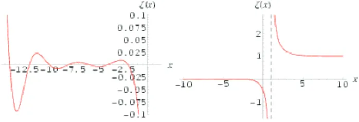
The case x= 1 is avoided since the series becomes divergent, Figure 1. For even powers the function gives exact values, proportional to even powers ofπ, as shown in (3.6); for odd powers it is not possible to get such an exact representations. The

Figure 1: Plot of the Riemann zeta function.

Bernoulli numbersBn are a set of rational numbers defined by the series [4]:

x e^x−1 =

∞

X

n=0

Bnxⁿ n! , B0= 1, B1=−1

2, B2= 1

6, B4=− 1

30, B6= 1

42, . . . (3.8) The zeta function is related with them for integer values of the argument xas:

ζ(n) = 2ⁿ⁻¹|Bn|πⁿ

n! , Bn= (−1)ⁿ⁺¹nζ(1−n), n∈N. (3.9)

4. The remainder term of Fourier series

The Fourier series develops a function by means of an infinite series of trigono- metric terms; its convergence is assured by Dirichlet conditions. However, in prac- tice, it is not possible to take an infinite number of such orthogonal functions, but a

The remainder term in Fourier series and its relationship with the Basel problem 21 finite number of them for performing a finite Fourier expansionfn(x), formed byn terms. Fourier series convergence shows that by taking a sufficiently large number of terms, the difference between f(x)and fn(x), named the remainder term, can be made as small as we desire:

ηn(x) =f(x)−fn(x). (4.1) Let us suppose thatf^(m)(x)exists, although its continuity is not demanded; how- ever, the continuity of f(x), f^′(x), f^′′(x), . . . , f^m−1(x) is required for setting the following boundary conditions:

f(π) =f(−π), f^′(π) =f^′(−π), . . . , f^m−1(π) =f^m−1(−π). (4.2) The existence of the above conditions let us simplify the integration of the coef- ficients in Fourier series, performed by parts successively m times. They can be gathered in a complex coefficient:

ak+jbk= j^m πk^m

Z π

−π

f^(m)(ξ)e^jkξdξ, (4.3) where the Fourier series is the real part of the series:

f(x) =

∞

X

k=1

(ak+jbk)e^−jkx= Z π

−π

f^(m)(ξ)

"

j^m π

∞

X

k=1

e^jk(ξ−x) k^m

#

dξ. (4.4)

The indexk= 0has been omitted sincef(x)stands forf(x)−a0/2. Let us change the integrating variable by θ= ξ−x, therefore, f(x)is written in terms of the kernel-type seriesGm(θ):

f(x) = Z π

−π

f^(m)(θ+x)Gm(θ)dθ, Gm(θ) = j^m π

∞

X

k=1

e^jkθ

k^m. (4.5) In the finite expansion fn(x), the kernel-type series must add only n terms, thus the remainder term is expressed in function of another kernel-type seriesg_n^m(θ):

ηn(x) = Z π

−π

f^(m)(θ+x)g_n^m(θ)dθ, g_n^m(θ) = j^m π

∞

X

k=n+1

e^jkθ

k^m . (4.6) The simpler method for getting the remainder term is based on Cauchy inequality:

"

Z b a

f(x)g(x)dx

#2

6 Z b

a

f²(x)dx Z b

a

g²(x)dx. (4.7) After applied it in (4.6) we get:

η_n²(x)6 Z π

−π

f^(m)2(θ+x)dθ Z π

−π

[g^m_n(θ)]²dθ. (4.8)

22 V. Barrera-Figueroa, A. Lucas-Bravo, J. López-Bonilla In this case, we can take advantage of the orthogonality of the members of the series g_n^m(θ), by taking their real part. The integral of the square of kernel-type series is:

Z π

−π

[g_n^m(θ)]²dθ= 1 π²

∞

X

k=n+1

Z π

−π

coskθ k^m

∞

X

l=n+1

coslθ l^m dθ= 1

π

∞

X

k=n+1

1

k^2m. (4.9) The above series seems to be related with the Riemann zeta function, however, we cannot get an exact result since the series starts from n+ 1. For estimation purposes, we can use the integral approach of a slow varying-type series, whose periodic part is the unitary function, i.e., α = 0. The slow varying part is the function ϕ(k) = 1/k^2m, which varies slowly, since m and n are supposed to be great:

1 π

∞

X

k=n+1

1 k^2m ≈ 1

π Z ∞

n+1/2

dξ

ξ^2m = 1

π(2m−1)(n+ 1/2)^2m−1. (4.10) The integral of f^(m)2, should be identified as the norm of the m^th derivative of f(x), represented by N_m², therefore the remainder term is bounded by:

|ηn(x)|< Nm

pπ(2m−1)(n+ 1/2)^m−1/2. (4.11) Another method for getting the remainder term is by evaluating reliably the kernel- type series g^m_n(θ)with the integral approach of a slow varying-type series, where the slow varying function corresponds with ϕ(k) = 1/k^m. With the exception of small values aroundθ= 0, we can use the asymptotic behavior of the integral:

g_n^m(θ)≈ j^mθ 2πsinθ/2

Z ∞ n+1/2

e^jξθ

ξ^mdξ≈ j^m+1 2πsinθ/2

e^j(n+1/2)θ

(n+ 1/2)^m. (4.12) For estimation purposes, the remainder term can be calculated by means the fol- lowing inequality:

|ηn(x)|6 Z π

−π|f^(m)(θ+x)||g_n^m(θ)|dθ=|f^(m)(x)|^max Z π

−π|g^m_n(θ)|dθ. (4.13) After taking the real part ofg_n^m(θ)and integrating it, we get the following formula:

|ηn(x)|< 2 (n+ 1/2)^m−1

ln(n+ 1/2)π

(n+ 1/2)π |f^m(x)|^max. (4.14)

5. Mean square error in Fourier series

Frequently the remainder term is known as the error term, for its interpretation is obvious. However, it is more suitable to handle a mean square error for practical issues:

η²= 1 2π

Z π

−π

η²_n(x)dx= 1 2π

Z π

−π

[f(x)−fn(x)]²dx. (5.1)

The remainder term in Fourier series and its relationship with the Basel problem 23 The orthogonality properties let us express the mean square error in function of the coefficients in Fourier series:

η²=1 2

∞

X

k=1

(a²_k+b²_k)−1 2

n

X

k=1

(a²_k+b²_k) =1 2

∞

X

k=n+1

(a²_k+b²_k), (5.2) where the mean square error results equal to the square of the remainder term:

η²= η²_n 2π

Z π

−π

dx=η²_n. (5.3)

The above formulae let us find out a relation between the norm of them^thderivative off(x)and the coefficients of its Fourier series. By substituting (4.9) into (4.8) we have:

η_n² 6 1 π

∞

X

k=n+1

1 k^2m

Z π

−π

f^(m)2(ξ)dξ, (5.4)

from which we get the following inequality:

1 2

∞

X

k=n+1

(a²_k+b²_k)6 1 π

∞

X

k=n+1

1 k^2m

Z π

−π

f^(m)2(ξ)dξ, (5.5) which provides us the wanted relation:

a²_k+b²_k < 1 πk^2m

Z π

−π

f^(m)2(ξ)dξ. (5.6)

If we consider that in the inequality (5.5) both series start from k= 1, we get:

1 2

∞

X

k=1

(a²_k+b²_k)6 1 π

∞

X

k=1

1 k^2m

Z π

−π

f^(m)2(ξ)dξ, (5.7) where the left side is proportional to the integral of f²(x):

∞

X

k=1

(a²_k+b²_k) = 1 π

Z π

−π

f²(x)dx, (5.8)

from which the following inequality is gotten:

1 2

Z π

−π

f²(x)dx6

∞

X

k=1

1 k^2m

Z π

−π

f^(m)2(ξ)dξ. (5.9) This series is expressed in terms of the zeta function, from which results the fol- lowing impressive inequality:

Z π

−π

f²(x)dx6 (2π)^2m (2m)! |B2m|

Z π

−π

f^(m)2(ξ)dξ. (5.10)