Topoligical Characterization of Cellular Structures

Topological Characterization of Cellular Structures

Tamás Réti

Budapest Polytechnic, Doberdó u.6, H-1031 Budapest, Hungary E-mail: reti@zeus.banki.hu

Károly Böröczky, Jr.

Alfréd Rényi Institute of Mathematics, P.O. Box 127, H-1364 Budapest, Hungary E-mail: carlos@renyi.hu

Abstract: In order to characterize quantitatively the local topological structure of cellular systems a new method has been developed. First, we analyzed the topological properties of infinite periodic cellular structures, and then the general theoretical results obtained have been adapted to the local topological characterization of 2-dimensional finite cellular surface systems. The concept of this new approach is based on the use of the so-called double toroidal embedding (DT embedding) by which a finite cellular system defined on a torus can be generated from an infinite periodic cellular system. The DT embedding is a special mapping, which enables to preserve all the local topological properties of the original infinite periodic cellular system. As a result of performing a DT embedding, so- called neighborhood coefficients can be generated. The neighborhood coefficients are scalar topological invariants, by which the local topological structure of cellular systems can be quantitatively evaluated and compared. Moreover, by investigating the relationship between the neighborhood coefficients and other local topological quantities, we verify that the validity of the Weaire-Fortes identity can be extended to a broad class of infinite periodic cellular systems and 2-d finite cellular surface systems (i.e. generalized fullerene- like surface structures). Finally, it has been shown that the traditional definition of fullerenes can be generalized by introducing the notion of the cellular fullerene, which is considered as a finite cellular system defined on a 2-d unbounded, closed and orientable surface.

Keywords: cell, embedding, toroidal graphs, Weaire-Fortes identity, corona, fullerene

1. Introduction

In various fields of material sciences, many interesting 2- and 3-dimensional structures (fullerenes, nanotubes, froths, metal foams, polycrystals) can be

modeled by a special arrangement of space filling polygons and polyhedra (i.e. 2- or 3- dimensional polytopes) and thus can be considered as finite or infinite cellular systems. Over the past two decades, most studies have concentrated on 2- d cellular structures which may be represented by infinite, planar networks, usually with trivalent vertices (i.e. three edges at each vertex) [1-6]. This paper presents a general method, which is designated primarily to the topological evaluation of infinite periodic and finite cellular systems composed of d- dimensional polyhedra (polytopes) where d ≥ 2.

The proposed method is based on the application of a double toroidal embedding (DT embedding) by which a finite space-filling cellular system defined on a torus can be generated. The DT embedding is considered as a one-to-one mapping of the topological types, which enables to preserve all the local topological properties of the original infinite periodic cellular system. It will be shown that, after performing a DT embedding, so-called neighborhood coefficients can be computed, by which the local topological structure of periodic cellular systems can be simply analyzed and compared. Additionally it will be verified that the validity of the Weaire-Fortes identity [2-4] playing a key role in the topological description of 2-dimensional random cellular patterns, could be extended to finite dimensional periodic cellular systems. The fundamental results concerning the extension of the Weaire-Fortes identity are represented by Eqs. (33 and 34).

Finally, it is shown that the traditional definition of fullerenes can be generalized by introducing the notion of the cellular fullerene, which is considered as a finite cellular system defined on a 2-d unbounded, closed and orientable surface.

2. Locally finite periodic cellular systems

The most important type of infinite d-dimensional cellular systems is the so-called countable cellular system [7]. A countable cellular system is considered as a face- to-face tiling (tessellation) of d-dimensional Euclidean space denoted by E^(d) by a countable set of d-dimensional compact combinatorial polyhedra (polytopes).

Each d-dimensional polyhedron called a cell is topologically equivalent (homeomorfic) to a d-dimensional sphere. A countable cellular system denoted by Ω_d is defined by taking into consideration the fulfillment of the following requirements:

i. Ωd can be represented as

⎪⎭

⎪⎬

⎫

⎪⎩

⎪⎨

⎧ ∈ =

= ^(d)

d E

Ω

∪

j j P

j j I ...and... A

A (1)

where IP is the index set of positive integers, Aj is the jth cell (polyhedron) in Ω_d.

ii. The k-dimensional faces of polyhedra included in Ωd (k=0,1,2,…,d-1) are also compact combinatorial polyhedra, and the maximum number of k-dimensional faces is less then γ_k, where γ_k are finite positive integers for k=0,1,2,…d-1. (The 0-dimensional and 1-dimensional faces of polyhedra are called vertices and edges, respectively.)

iii. Polyhedra can be included in a d-dimensional sphere with a finite radius, which guaranties that the “size” of cells is finite [7].

iv. All of the k-dimensional faces of a d-dimensional polyhedron have a positive k-dimensional volume (measure) for k=1,2,…d.

v. Each (d-1) -dimensional face between cells is the common face of two different cells (polyhedra) exactly.

vi. Additionally it is assumed that Ωd is locally finite [7]. By definition, a countable cellular system is called locally finite if there exists a positive number ρ for any arbitrary point Px in E^(d), such that every d-dimensional sphere G(Px,ρ) with radius ρ and center point Px, contains finite number cells from Ωd only. This definition implies that there are no singularity points of cells in the cellular system. For each vertex X (0-dimensional face) in Ω_d the number of edges (1- dimensional faces) incident to X is called the valency of X, denoted by r (or r(X)).

If all of the vertices of have the same valency R, then Ωd is said to be a regular, or R-valent cellular system.

For purposes of our investigations the most important groups of locally finite cellular systems are the periodic cellular systems. A locally finite cellular system Ωd is called periodic, if there exists a d-dimensional parallelepiped Πd represented by a linearly independent vector system (v1, v2,… vk, ....vd) for which relationships

{

d

}

d

Ω

Π ⊂ ∪ A

_j

A

_j

∈

(2a) and

⎪⎭

⎪ ⎬

⎫

⎪⎩

⎪ ⎨

⎧ = + ε ε ∈

=

_ε

∑

^d=

^,...

^k

^I

1

k k k d

v v

(d)

B B Π v

E ∪

(2b)

are fulfilled, where ε_k are integers for k = 1,2,….d, and Iε is the set of integers [7].

In the following, it is supposed that Ωd is a locally finite periodic cellular system (LFPC system). From the previous considerations it follows, that parallelepiped Π_d can be covered by the union of a finite set of cells belonging to Ω_d. This implies that a LFPC system is generated from a finite set of polyhedra of combinatorially different types.

It will be shown that the topological description of a locally finite periodic cellular system (LFPC system) can be traced back to the topological characterization of an appropriately constructed finite cellular system. Parallelepiped Πd has been chosen in such a way, that it has a minimum volume. It should be emphasized that this parallelepiped Π_d is not uniquely defined. They can be constructed in different manners; however, their common property is that their d-dimensional volumes are identical.

There is no loss in generality in assuming the following: By using an appropriately selected homogenous linear transformation, parallelepiped Π_d can be mapped into a d-dimensional unit cube. This unit cube Π_d,U which is called “a unit domain” in the classical crystallography is given by

Π_d,U = {x = (x₁, x2,…xk,…xd) | 0 ≤ x_k ≤ 1 and k = 1,2,…d} (3) This simple transformation makes it possible to replace the original LFPC system

by a “standardized” periodic cellular system generated by translations of Πd,U. The only difference is that the standardized LFPC system is composed of unit cubes instead of parallelepipeds. Since a linear transformation represents a “topology preserving” onto-to-one mapping, this implies that the original and the transformed periodic cellular systems are topologically equivalent. In the further investigations, it will be supposed that the LFPC system Ω_d is a standardized cellular system.

3. Finite cellular systems constructed by using a double toroidal embedding

From a LFPC system, finite cellular systems of a toroidal type can be constructed in several ways. In the following, it will be demonstrated that starting with a d- dimensional LFPC system and by using the so-called double toroidal embedding, it is always possible to construct a uniquely defined finite cellular system represented by a torus in the (d+1) dimensional Euclidean space, which is advantageously applicable to the local topological evaluation of infinite periodic cellular systems.

In order to generate a finite cellular system from a standardized LFPC system, consider a unit domain Πd,U defined by Eq. (3). As a first step, let us construct a so-called identification region Sd, which is composed of 2^d unit domains, as follows

Sd = {x = (x₁, x2,…xk,…xd) | 0 ≤ x_k ≤ 2 and k = 1,2,…d} (4) As can be stated, Sd is also a d-dimensional cube with edge length of 2. As a

second step, let us construct a finite toroidal cellular system Rd (FTC system) by

gluing (identifying) the opposing k-dimensional face pairs (edges, vertices, etc.) of Sd (k=0,1,2,….d-1).

Fig.1 The 3-dimensional, periodic Weaire-Phelan cellular system This mapping is called the double toroidal embedding (DT embedding) of the d- dimensional LFPC system, because Rd represents a torus in the (d+1)- dimensional Euclidean space. As an example, Fig. 1 shows a two-component, space-filling periodic polyhedral system. In this 3-dimensional LFPC system that was discovered by Weaire and Phelan, the space-filling unit domain consists of six tetrakaidecahedra (14-sided Goldberg polyhedra) and two irregular pentagonal dodecahedra (12-sided polyhedra) [8].

Fig.2 Identification region S3 generated by 8 unit domains to the DT embedding of a 3-d LFPC system

In Fig. 2, the construction of the identification region of a 3-dimensional LFPC system is illustrated. As can be seen, this is the union of 8 unit domains. The

arrows a, b and c are used to specify a direction for the edges, and this direction must be respected when gluing is done. The eight vertex points of the identification region S3 are joined to form a single point ω of the resulting toroidal system.

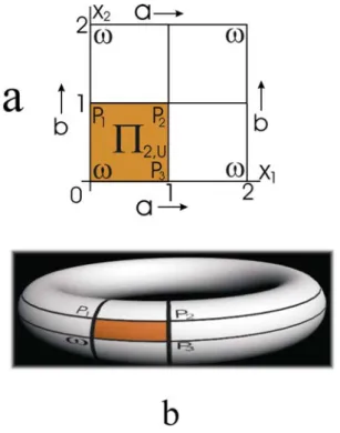
Fig. 3 demonstrates the general concept of the DT embedding of a 2-dimensional LFPC system. As an example, in Fig. 4., the DT embedding is shown for a 2-d periodic cellular system, which includes 4- and 8-sided polygons. The resulting FTC system is also composed of four 4-sided and four 8-sided cells (See Fig 4.c).

The number of cells is 8, the number of edges is 24, and the number of vertices is 16. As it is expected, the Euler-characteristic of this finite system defined on the torus surface is zero.

Fig.3 Principle of the DT embedding of a 2-d LFPC system (a) The 2-d identification region S2 composed of 4 unit domains, (b) The corresponding FTC

system defined on a torus

Fig.4 Example of the toroidal embedding of a 2-d LFPC system (a) The unit domain Π2,U, (b) The corresponding identification region S2, (c) The DT embedding performed on the torus, (d) The traditional toroidal embedding of the

2-d LFPC system by using a single unit domain only

The basic properties of the DT embedding and of FTC systems are as follows:

a. The total number of cells in Sd is equal to Nd,U x 2^d, where Nd,U denotes the number of cells in the unit domain.

b. The resulting FTC system preserves all the topological properties of the original LFPC system. This is due to the following fact: In cellular systems generated by a DT embedding, each (d-1)-dimensional face is shared by two different neighbor cells exactly. Since a DT embedding is a topology preserving one-to-one mapping between the LFPC and FTC

system this implies that an LFPC system can be unambiguously reconstructed from the corresponding FTC system generated by a DT embedding. It should be noted, that using a single unit domain could also perform a toroidal embedding. Unfortunately, in certain cases, if we use only one unit domain to generate a finite toroidal cellular system, as a result of this procedure the local topological properties characterizing the neighborhood structure of cells can change radically. Consequently, the classical toroidal embedding cannot be applicable to every case. As an example, this is illustrated in Fig 4.d. Due to the toroidal embedding with a single unit domain, the original topological structure of the 2- dimensional LFPC system depicted in Fig. 4.a, has been degenerated. In this case, the number of cells is 2, the number of edges is 6, and the number of vertices is 4, the Euler-characteristic is zero. As it can be stated Fig 4.d shows the conventional 2-cell embedding of the complete graph K4 in the torus, where one of the two cells is 4-sided, while the other is 6-sided. This is explained by the fact that in this toroidal cellular system there exist two edges, which belong to the same 6-sided cell. This implies that the original LFPC system shown in Fig. 4.a, cannot be reconstructed from the finite graph depicted in Fig 4.d.

c. Every FTC system generated by the DT embedding of a 2-dimensional LFPC system can be represented by a finite toroidal graph. (i.e. 2- dimensional FTC systems are considered as a subset of toroidal graphs).

This implies that the topological analysis of 2-dimensional LFPC systems can be reduced to the characterization of traditional toroidal graphs embedded on a genus 1 surface.

4. Topological properties of FTC systems

In order to simplify the treatment of problems to be outlined, we introduce some definitions. Let us denote by Nd,k the number of k-dimensional faces of FTC system Rd where k=0,1,2,…d. By definition, Nd,d is the number of cells (polyhedra), Nd,0 is the total number of vertices, Nd,1 is the total number of edges, Nd,2 is the total number of traditional faces of cells.

The finite toroidal cellular system Rd generated by space filling polyhedra (polytopes) can be represented as

Rd = {An,i⏐i=1,2,..N_n, nmin ≤ n ≤ n_max, n∈ I_R}. (5) In Eq.(5), An,i denotes the ith cell (d-dimensional polyhedron) with n-faces, where

i= 1,2,...Nn and Nn is the total number of d-dimensional, n-faceted cells in Rd. By definition, an n-faceted cell stands for a d-dimensional cell having (d-1)

dimensional faces of number n. It is supposed that nmin≥2 and nmax >nmin are positive integers, IR is a finite index set for n.

The total number Nd,d of cells is Nd,d=

∑

^Nn where n=2,3,... nmax. The fraction (or frequency) pn of n-faceted cells is pn = Nn/Nd,d , where pn>0. Consequently,

∑

^pn=1. For a FTC system, the mean number of (d-1) dimensional faces per cell denoted by 〈n〉 can be calculated as^〈n〉=

∑

^npn. Generally, in the cell statistics, expression 〈U(n)〉 is the average value of the quantity U(n) with frequency pn, i.e. ^〈U(n)〉=

∑

^pnU(n) by definition.

Since any (d-1) dimensional face is a common face of two different neighbor cells, this implies that

d , d

1 d , d d

, d n

n

n

n

N

N 2 N

nN 2 np

n 〉 = = =

⁻

〈 ∑

∑

⁽⁶⁾

and

∑∑ ∑∑

≤ −

≥ −

−

= =

n k n

1 d , d n k n

1 d 1

d

( n , k ) e ( n , k ) N

e

(7)

where Nd,d-1 is the total number of (d-1) dimensional faces, and ed-1(n,k) is the number of the common (d-1) dimensional faces of n-faceted and k-faceted neighbor cells.

In a FTC system, vertices do not all have the same valency, consequently, we may define an average valency [r] as follows:

∑

=

r ) d ( r 0 , d

N rV ] 1 r

[ (8)

where

V

_r^(d) is the number of r-valent vertices in Rd and ⁼

∑

r ) d ( r 0

,

d V

N . For

every FTC system we have

∑

=

=

r ) d ( r 0

, d 1

,

d [r]N rV

N

2 (9)

which is due to the fact, that each edge has two different ends (endvertices).

The component number of a FTC system is defined by ^Φ=

∑

^{sgn(pn). It}

follows from the definition that Φ≥1. On the other hand, Φ=1, if and only if the FTC system is a so-called face-homogenous system which is composed only of

polyhedra with identical face numbers. It should be noted that there exist face- homogenous LFPC systems including combinatorially different cells (i.e.

topologically non-equivalent polyhedra) with identical face numbers. (The simplest 3-dimensional LFPC system of such type is composed of two combinatorially different 5-sided polyhedra.)

4.1 Euler-equation for FTC systems

It is has been shown, that the traditional Euler-formula can be extended to the topological description of FTC systems [7, 9-11]. This modified Euler-equation, which valid even for a d-dimensional FTC system can be formulated as follows:

For an arbitrary FTC system Rd where all the k-dimensional faces are topologically equivalent to a k-dimensional sphere, the equality

( ) ∑ ( )

=

=

−

=

χ

^d

0 k

k , d

k

N 0

d

1

R

(10)

is valid. In Eq.(10), χ(R_d) is the Euler-characteristic of the finite toroidal cellular system Rd. Particularly, for the case of d=2, we have

0 N N

N

_2,2

−

_2,1

+

_2,0

=

(11)

while for the case of d=3,

0 N N N

N

_3,3

+

_3,2

−

_3,1

+

_3,0

=

−

(12)

yields.

Because the unit domain Πd,U representing the corresponding LFPC system has a minimum volume, it follows that the total numbers of k-dimensional faces in Rd (k=0,1,2,…d), i.e. quantities Nd,k in Eqs. (10-12) are uniquely defined positive integers.

For the 2-dimensional case, identity (11) coincides with Euler’s theorem for the torus [7,9]. For the 3-dimensional case, Eq.(12) has been proven by Kinsey [10], who verified that if R3 is a compact connected 3-manifold without a boundary then χ(R₃) = 0. The proof of the general case is based on the following concept:

Considering the Euler-characteristic of a d-dimensional torus, we argue as follows: The d-dimensional torus can be represented as the direct product of d circles (meaning d circular arcs). Since the Euler-characteristic is multiplicative with respect to direct products and the Euler-characteristic of a circle is zero, this implies that the Euler-characteristic of a d-dimensional torus is zero, as well. (See Exercise B4 on page 205 in Ref. [11]).

4.2 Cell coronas

The analysis of local topological properties can be traced back to the evaluation of the correspondences between the individual cells and their first neighbor cells.

Cells A and B are called adjacent (neighbors) if they have common (d-1) dimensional faces. The cell corona C(A) of a cell A in Rd is the union of neighbor cells of A. According to this definition, cell A is not included in C(A).

FTC systems can also be characterized on the basis of the topological properties of their cell coronas. For this purpose, we define the corona frequency vector fA (CF- vector) of cell A included in Rd as follows:

(

n^(A_max⁾

)

) A ( k ) A ( 3 ) A (

2

, f ,... f .... f

= f

f

A (13)

where component f_k^(A) is the number of (d-1) dimensional, k-faceted cells in C(A), and index nmax denotes the maximum (d-1) dimensional face number of cells included in Rd. It is obvious that for any k and f_k^(A)relationships 0≤ f_k^(A) ≤ nmax and nmin=2≤ k ≤nmax are valid, and f_k^(A)= 0 if and only if, there is no k- faceted neighbor cell in C(A). It is clear that, if A is an n-faceted cell, then the sum of components of fA is equal to n.

Consider two n-faceted cells An and Bn characterized by their corresponding CF- vectors denoted by fA,n and fB,n. Cells An and Bn are called topologically similar, if fA,n≡fB,n is fulfilled. As can be stated, this topological similarity is an equivalence relation by which all the cells of a FTC system can be classified into disjoint subsets.

This implies that all the topologically similar n-faceted cells denoted by

j) , Rn (

j , n ) 2 (

j , n ) 1 (

j ,

n ,A ,...,A

A are the elements of the same configuration set Rn,j

defined as

Rn,j

{

⁽n^R,j^n,j)

}

) 2 (

j , n ) 1 (

j ,

n

, A ,...., A

= A

(14)

where Rn,j is the number of topologically similar n-faceted cells in Rn,j

(j=1,2,…J(n)). It follows that Rd can be described as a union of disjoint subsets

∪ ∪

n ) n ( J

j=1

=

_n,j

d

R

R

(15)

where J(n) stands for the number of configuration sets including topologically similar, n-faceted cells. It is obvious that cells belonging to Rn,j is characterized by

the same FC-vector

f

_Rn,j. Let us denote by pn,j the fraction of topologically similar n-faceted cells included in Rn,j. Because pn,j= Rn,j/Nd,d it follows that

1 p p

n n

n )

n ( J

1 j

j ,

n

= =

∑ ∑ ∑

=

(16)

It is easy to see that pn,j and

f

_Rn,jare unambiguously defined quantities which are independent of the particular choice of the unit domain of the LFPC system. It follows that the total number J of possible configuration sets Rn,j can be calculated as

∑∑

∑ ⁼

=

n j

j , n n

) p sgn(

) n ( J

J

(17)

It is obvious that for any FTC system inequality J≥Φ is fulfilled. This means that the total number of possible configuration sets is not less than the component number Φ of the FTC system. The quotient ϕ=Φ/J ≤1 which is called the complexity index of the cellular system, gives information on the fraction of topologically distinct cell coronas in the LFPC and the corresponding FTC system.

4.3 Face-coordination number

The face-coordination number mA of an arbitrary n-faceted cell A belonging to the configuration set Rn,j is defined as

∑

=

k

j) , Rn ( k

A

kf

n

m 1

(18)

where

f

_k^(Rn,j) is kth component of the CF-vector

f

_Rn,j.

The face-coordination number mA is the mean number of (d-1) dimensional faces of the neighbors of A. It should be emphasized that mA is a local topological parameter, which gives some information on the arrangement of the cells included in the cell-corona. For the FTC system Rd which is composed of cells An,i

(i=1,2,..Nn), the mean face-coordination number m(n) of n-faceted cells is defined as

∑

=

=

^Nn

1 i An,i n

N m ) 1 n (

m

(19)

where

m

_An,i is the face coordination number of cell An,i.

Knowing the set of FC-vectors

f

_Rn,j and the corresponding fractions pn,j of topologically similar cells, the mean face-coordination number m(n) of n-faceted cells can be calculated as

∑ ∑

=

⎭ ⎬ ⎫

⎩ ⎨

=

^J(n)

⎧

1

j k

j) , Rn ( k j

, n n

kf np p

) 1 n (

m

(20)

Starting with Eqs.(19 and 20) we define the total face-coordination number 〈m(n)〉

of Rd as follows

∑ ∑ ∑

∑

=

⎭ ⎬ ⎫

⎩ ⎨

= ⎧

=

n ) n ( J

1

j k

j) , Rn ( k j

, n n

n

p kf

n ) 1 n ( m p )

n (

m

(21)

It is conjectured that for all FTC systems inequality 〈m(n)〉 ≥ 〈n〉 holds, and

〈m(n)〉 = 〈n〉 if and only if, the cellular system is a face-homogenous system including cells with identical face numbers only (i.e. Φ = 1 is fulfilled).

4.4 Neighborhood coefficients

Now, let us define quantities denoted by H(n,k) as

j) , Rn ( k ) n ( J

1 j

j , n

f p )

k , n (

H ∑

=

=

(22)

where nmin ≤ n,k ≤ n_max. Quantities H(n,k) are called the neighborhood coefficients of the FTC system. The neighborhood coefficients are non-negative numbers, which have a special property of symmetry

) n , k ( H f

p f

p )

k , n (

H

_n^(Rk,j)

) k ( J

1 j

j , k j)

, Rn ( k ) n ( J

1 j

j ,

n

= =

= ∑ ∑

=

=

(23) The neighborhood coefficients can be interpreted geometrically as follows:

⎪ ⎪

⎩

⎪ ⎪

⎨

⎧

=

≠

=

−

−

k n if ) n , n ( N e

2

k n if ) k , n ( N e

1 )

k , n ( H

1 d d , d

1 d d , d

(24)

where Nd,d is the number of d-dimensional cells, and ed-1(n,k) is the number of the common (d-1) dimensional faces of n-faceted and k-faceted neighbor cells.

Especially, for the case of d=2, we have

⎪ ⎪

⎩

⎪ ⎪

⎨

⎧

=

≠

=

k n if ) n , n ( N e

2

k n if ) k , n ( N e

1 ) k , n ( H

1 2 , 2

1 2 , 2

(25)

where N2,2 is the number of 2-dimensional cells (polygons), and e1(n,k) is the number of the common edges (i.e. 1-dimensional faces) of n-sided and k-sided neighbor cells.

For the case of d=3,

⎪ ⎪

⎩

⎪ ⎪

⎨

⎧

=

≠

=

k n if ) n , n ( N e

2

k n if ) k , n ( N e

1 ) k , n ( H

2 3 , 3

2 3 , 3

(26)

where N3,3 is the number of 3-dimensional cells (polyhedra) and e2(n,k) is the number of the common 2-dimensional faces of n-faceted and k-faceted neighbor polyhedra.

It is easy to verify, that for quantities H(n,k) the following relationships are valid:

∑

∑ ⁼

=

k k

n

H ( k , n )

n ) 1 k , n ( n H

p 1

(27)

∑

∑ ∑

⁼

⎭⎬

⎫

⎩⎨

⎧

n z z n n

z

k

n p )

k , n (

H (28)

1 z 1 z

n n

n

n k

z k

z

H ( n , k ) n H ( n , k ) p n n

k = =

⁺

=

⁺

∑ ∑ ∑ ∑ ∑

⁽²⁹⁾

where z is an arbitrary integer. Additionally, from Eq.(6), identity

1 d , d d

, d

n k

d ,

d

H ( n , k ) N n 2 N

N ∑∑ = =

₋ ⁽³⁰⁾

yields. For the case of d=2 we have

∑∑

∑∑

≤

=

=

=

n k n 1 1

, 2 2

, 2

n k

2 ,

2

H ( n , k ) N n 2 N 2 e ( n , k )

N

(31)

where N2,1 is the total number of edges (i.e. 1-dimensional faces) and 〈n〉 is the mean number of edges per cell in R2. For the case of d=3

∑∑

∑∑

≤

=

=

=

n k n 2 2

, 3 3

, 3

n k

3 ,

3

H ( n , k ) N n 2 N 2 e ( n , k )

N

(32)

yields, where N3,2 is the total number of 2-d faces and 〈n〉 is the mean number of faces per cell in R3. As an example of application of these ideas, we consider the 3-dimensional, periodic Weaire-Phelan cellular system shown in Fig.1. This 2- component and 4-valent polyhedral system (i.e. Φ=2, R=4) consisting of 12- and 14-sided polyhedra is characterized by the following topological quantities:

p12=1/4, p14=3/4, 〈n〉=27/2=13.5, 〈n²〉=183, ϕ=Φ/J=2/3=0.667, H(12,12)=1, H(12,14) = H(14,12)=2 and H(14,14)=17/2=8.5.

5. A fundamental property of LFPC and FTC systems

Neighborhood coefficients H(n,k) play a key role in the topological characterization of LFPC systems. In the following a fundamental property of LFPC and FTC systems will be presented which can be formulated in the following statements:

On the one hand

( )

∑∑

≤ −

−

+ 〉 = 〈 〉 +

〈

n k n

1 d z z 1

d , d 1

z n k e (n,k)

N 2

n n (33)

on the other hand

〉

〈

=

〉

〈 n

^z+1

nm ( z , n )

(34)

where z is an arbitrary integer, and

∑ ∑

=

⎭ ⎬ ⎫

⎩ ⎨

=

^J(n)

⎧

1

j k

j) , Rn ( k z j , n n

f k np p

) 1 n , z (

m

(35)

by definition. As it can be stated, Eq. (35) is the generalization of Eq.(20). As a special case, when z=1, from Eq.(35) we obtain the mean face coordination number m(n) of n-faceted cells which is defined by Eq.(20). Consequently, identity m(n)=m(1,n) is fulfilled.

Proof of Eq. (33) is based on the following concept. Starting with Eqs.(24 and 29), we have

{ }

∑

∑

∑

∑

∑ ∑

∑

∑ ∑

∑

∑∑

≥

−

>

−

>

−

−

≠ −

−

≠ +

+

=

⎪⎪

⎭

⎪⎪⎬

⎫

⎪⎪

⎩

⎪⎪⎨

⎧

+ + +

⎭=

⎬⎫

⎩⎨ + ⎧

⎭=

⎬⎫

⎩⎨ + ⎧

=

=

〉

〈

k n

k , n

1 d z z d

, d

k n

k , n

1 d z

k n

k , n

1 d z d

, d

z z n

1 d d , d

k

n k

1 d z d

, d n

1 d z d , d

k

n k

z n

z

n k

z 1

z

) k , n ( e ) k n N (

1

) k , n ( e k ) k , n ( e N n

1

n n ) n , n ( N e

1

) k , n ( e N k

) 1 n , n ( e N n

2

) k , n ( H k )

n , n ( H n

) k , n ( H k n

(36)

Additionally, from Eq. (30) it follows

〉

= 〈

⁻

n N

N

_d,d

2

^{d,d 1} (37)

Substituting Eq.(37) into Eq.(36) we have

∑∑

≤ − + −

⎟⎟⎠

⎜⎜ ⎞

⎝

⎛ +

〉

〈

=

〉

〈

n k n

z z

1 d , d 1 1 d

z

2 k n N

) k , n ( n e

n (38)

It is important to note that Eq.(38) can be interpreted geometrically as follows: Let us denote by q(n,k)=ed-1(n,k)/Nd,d-1 the relative frequency of the common faces of n-faceted and k-faceted neighbor cells, for which

∑

^q(n,k)=1. Additionally, let us define quantities denoted by w(z,n,k)= (n^z + k^z)/2, which are considered as

positive weights belonging to the (d-1) dimensional common face of n- and k- faceted neighbor cells. Now, Eq.(38) can be rewritten in the form

∑ ∑

≤ + 〉 =〈 〉

〈

n k n 1

z n q(n,k)w(z,n,k)

n (39)

It is worth noting, when z = -1, from Eqs.(37 and 38) the identity

⎟⎠

⎜ ⎞

⎝⎛ +

=

∑ ∑

≤ −

k 1 n ) 1 k , n ( e N

n k n 1 d d

,

d (40)

yields.

The second statement represented by Eq.(34) can be proved as follow: By using Eq.(35) and Eq.(23) incorporating the definitions of quantities m(z,n) and H(n,k), we have

〉

〈

⎭=

⎬⎫

⎩⎨

= ⎧

⎪⎭

⎪⎬

⎫

⎪⎩

⎪⎨

⎧

⎪⎭

⎪⎬

⎫

⎪⎩

⎪⎨

⎧

⎭=

⎬⎫

⎩⎨

= ⎧

〈

+

=

=

∑ ∑

∑ ∑ ∑

∑∑ ∑

1 z

n k

z n

) n ( J

1 j

j) , Rn ( k j , n k

z n

) n ( J

1

j k

j) , Rn ( k z j , n

n ) k , n ( H k f

p k

f k p

) n , z ( nm

(41)

In particular cases, when z =1, from Eq.(41) we obtain the well-known identity formulated as 〈nm(n)〉 = 〈n²〉 which were considered by Weaire and Fortes [2,3]

for random 2-d cellular systems, and by Fortes for random 3-d cellular systems [4].

In the following it will be demonstrated that the general concept used for the topological description of locally finite periodical cellular systems can be efficiently applicable to the structural characterization of fullerene solids represented by finite cellular surface systems.

6. Cellular fullerenes

The discovery of fullerene molecules and related forms of carbon such as nanotubes has generated an explosion of activity in physics, chemistry and material science. As it is known, the topological properties of fullerenes play a key role in a classification of possible fullerene structures and in predicting their various physical and chemical behaviors.

In chemistry, the traditional definition is that a fullerene is an all-carbon molecule in which the atoms are arranged on a pseudospherical framework made up entirely of hexagons and pentagons. Based on the concept outlined in Refs. [12-14], define a fullerene in the wider sense as follows: A fullerene is considered as a simple finite cellular system (SFC system) defined on an unbounded, closed and oriented surface, and composed of a finite set of combinatorial polygons (called cells), where cells are simply connected regions and all common edges are shared only by two different neighbor cells. Fullerenes of such types will be referred to as cellular fullerenes. According to this general definition, the closed nonotubes with negative curvature and the so-called onion-like structures are also considered as fullerenes [13,14]. Taking into consideration the decisive role of the Euler characteristic (χ) in the topological analysis of unbounded, closed and oriented surfaces, cellular fullerenes with χ=2 are called spherical, while cellular fullerenes with χ=0 are called toroidal fullerenes.

6.1 Non-polyhedral spherical fullerenes

Cellular spherical fullerenes generated by the tessellation of the surface of the unit sphere can be classified into two classes. Spherical fullerenes represented by convex polyhedra are called polyhedral fullerenes, while the others, which cannot be represented by convex polyhedra, are called non-polyhedral fullerenes. It should be noted that, the Schlegel diagram of a polyhedral fullerene is considered as a polyhedral graph. According to the Steinitz’s theorem, a finite graph is polyhedral if and only if it is planar and 3-connected [16]. This implies that the Schlegel diagram of a non-polyhedral spherical fullerene is represented by a 2- connected graph. It is important to note, that among the spherical fullerenes there exist several topologically distinct isomers, which can be of polyhedral and non- polyhedral types.

Fig.5 Schlegel diagrams of non-polyhedral, trivalent fullerenes: (a) a generalized triangular T8,is fullerene with 8 vertices, (b) a generalized triangular T12,is

fullerene with 12 vertices

Deza et al. investigated some special types of polyhedral fullerenes, namely, the so-called triangular fullerenes composed of triangles and hexagons only [15]. A triangular fullerene is defined as a simple polyhedron with trivalent vertices, for which the k vertices are arranged in 4 triangles and (k/2-2) hexagons (and 3k/2 edges). Triangular fullerenes denoted by Tk can be constructed for all k≡0 (mod 4) except k=8. Examples of such polyhedra are the tetrahedron T4,the truncated tetrahedron T12 and the chamfered tetrahedron T16 [15]. By extending the definition of triangular fullerenes we can construct spherical and trivalent isomers, which are of non-polyhedral types. In Fig.5 the corresponding Schlegel diagrams of two non-polyhedral triangular fullerenes denoted by T8,is and T12,is are shown.

It is worth noting that T8,is is the smallest non-polyhedral trivalent fullerene because T8,is has no isomers of polyhedral types.

6.2 Global topological properties of cellular fullerenes

In a SFC system, the total number E of edges is related to the total number Nt of cells, the number V of vertices, the average valency [r] and the mean number of sides per cell 〈n〉

V ] r [ rV N

n nN E

2

r r n

t

n

∑

∑ ^{= = =}

=

(42)

where Nn is the number of n-sided polygons. The number V of vertices is V=

∑

^{Vr where Vr} is the number of r-valent vertices, the total number Nt of cells

(polygons) is Nt=

∑

^Nn where n=2,3,... nmax, and the fraction pn of n-sided cells is pn=Nn/Nt, for pn>0.

Assuming that all the cells are simply connected regions, Euler’s equation can be formulated as

g 2 2 V E

N

_t

− + = −

=

χ

(43)

where χ is the Euler-characteristic, g is the genus of the surface [16]. The genus of the surface, which can be an arbitrary non-negative integer, is identical to the number of handles that are attached to the sphere to obtain a surface. For the sphere χ=2 and g=0, for the torus (donut) χ= 0 and g=1, for the double torus, χ = - 2 and g=2, for the triple torus, χ = -4 and g=3, respectively. It is worth noting that identity (43) is a possible generalization of Eq.(11), because for the torus (where equalities χ=0 and g=1 are fulfilled), from Eq.(43) we obtain Eq.(11) as a special case. Taking into consideration, that for a SFC system equalities 〈n〉 = 2E/Nt and [r]= 2E/V are fulfilled, from Eqs.(42 and 43), we have

E 2 2 1 E

g 1 2 1 n 1 ] r [

1 + = + − = + χ . (44)

Additionally, from Eqs. (42 - 44) it follows

E 1 V 1 N N 2

2 1 ] r [

] r [

n 2

^t

t

−

− χ

⎭ =

⎬ ⎫

⎩ ⎨

⎧ − χ

= −

(45)

( ^{[ r ] 2} ) ^{/ 2}

V

N

_t

= χ + −

(46)

and

( ) ( )

V V 2 E V 2 N u 2 r V

2 V r

1

_t

r

r r

r

= − χ

= −

−

=

− ∑

∑

⁽⁴⁷⁾

where ur =Vr/V is the fraction of r-valent vertices, for which

∑

^{ur =1 and}

∑

^{rur =[r]} are fulfilled. An immediate consequence of Eq.(45) is that for trivalent SFC systems, equality 〈n〉=6(1-χ/N_t) = 6-12χ/(2χ+V) is valid. Depending on the particular choice of the Euler–characteristic χ, as particular cases, we get

〈n〉<6 for a sphere (case χ=2), 〈n〉=6 for a torus (case χ=0) and 〈n〉>6 for a double torus (case χ=-2), respectively.

6.3 Local topological properties of cellular fullerenes

First of all, it is important to emphasize that general formulae derived for d- dimensional LFPC systems (see formulae given by Eqs.(6 - 41)) can be applied to arbitrary fullerenes represented by simple finite cellular systems. It is easy to see that the fundamental identities given by Eqs.(33 and 34) remain valid for any SFC system (i.e. for cellular fullerenes).

In the following, by introducing the notion of the so-called vertex corona, we will demonstrate that the vertex corona distribution can be efficiently used to the local topological characterization of regular (R-valent) cellular fullerenes represented by SFC systems.

In a SFC system, cells A and B are called diagonally adjacent (diagonal neighbors) if they have a common vertex X. Vertex corona CV(X) of an arbitrary vertex X is defined as a union of diagonal neighbor cells having a common vertex X. For a finite cellular system characterized by the sequence of vertices Xk (k

=1,2, …V)

∪

j

k j k

V

( X ) A ( X )

C =

(48)

where Xk is a common vertex of cells Aj(Xk).

Vertex corona distribution of a cellular fullerene represented by a regular SFC system has an interesting property. Consider a finite cellular system, where Xr,k

denotes the kth and r-valent vertex, and define the topological quantity

∑

=

=

^V

1 k

v

M ( r , k )

V

M 1

(49)

where M(r,k) stands for the mean number of sides of cells in CV(Xr,k) for k = 1,2,…V. The local topological parameter M(r,k) is called the vertex coordination number of Xr,k while Mv is said to be the total vertex coordination number of the FTC system.

Now, we will verify that for regular, R-valent FTC systems (i.e. cellular fullerenes), identity

v

2 n M

n 〉=〈 〉

〈 (50)

is valid. Proof of Eq. (50) is based on the following considerations: Let us denote by

n ( B

⁽_j^k)

)

the side number of cell

B

⁽_j^k) belonging to the vertex corona CV(XR,k), where k = 1,2,…V and j=1,2,…R. It follows that

{ ^{n ( B ) n ( B ) ... n ( B ),... n ( B )} }

R ) 1 k , R (

M =

₁^(k)

+

⁽₂^k)

+

⁽_j^k)

+

⁽_R^k) (51)

Starting with Eq.(51), we have

∑∑ ∑

∑

= = =

=

=

=

= ^V

1 k

R

1

j n

n 2 )

k ( j V

1 k

v n N

VR ) 1 B ( VR n

) 1 k , R ( V M M 1

∑ ^{= 〈 〉 = 〈} _{〈 〉} ^〉

=

n

2 t 2

n t 2

n n n

E 2 p N VR n

N

(52)

It is easy to see that formula (50) can be generalized as follows: If z is an arbitrary integer, then identity

) z ( M n n^{z 1}〉 =〈 〉 _v

〈 ⁺ (53)

is valid for regular SFC systems, where

∑

=

=

^V

1 k

v

M ( R , k , z )

V ) 1 z (

M

(54)

and

{ ^{n ( B ) n ( B ) ,... n ( B )} }

R ) 1 z , k , R (

M =

^z ₁^(k)

+

^{z (}₂^k)

+ +

^{z (}_R^k) (55)

by definition. As it can be stated, when z = 1, this implies that Eq. (53) is simplified to Eq. (50). This is due to the fact, in the case of z=1, it follows that M(R,k,1)= M(R,k) and MV(1) = MV, respectively.

For trivalent and 2-component cellular fullerenes, (i.e. for the case of Φ=2 and R=3), which include α-sided and β-sided cells with frequencies pα and pβ = 1- pα (where α<β), there exist only four possible types of vertex coronas denoted by Cα,α,α, Cα,α,β, Cα,β,β and Cβ,β,β respectively. This implies that in this particular case, Eq.(50) can be reduced to the form

〉

〈

〉

= 〈 +

+ +

= n

M n s M s M s M s M

2 4 4 3 3 2 2 1 1 v

(56) where M1=(α+α+α)/3, M₂=(α+α+β)/3, M₃=(α+β+β)/3 and M₄ =(β+β+β)/3 are

the vertex coordination numbers of the four possible types of vertex coronas, and si (i=1,2,3,4) are the corresponding relative fractions of the vertex coronas, for which

∑

^{si =1} holds. Using identity (56) facilitates the computation of vertex fractions si (i=1,2,3,4), which are topological invariants. (For example, if quantities s1 and s2 are known, then s3 and s4 can be directly calculated.)

Fig.6 The four possible vertex coronas in a 2-component, trivalent fullerene (case α=5 and β=6).

6.4 Application: Topological characterization of C

60

fullerenes

As we have mentioned previously, the analysis of the distribution of vertex coronas of different types plays a significant role in algorithms for the perception and classification of topological properties of fullerenes. Balaban et al. have used this concept in order to classify the C60 isomers on the basis of topological properties of their vertex coronas [17]. Since C60 fullerene isomers are composed of 12 pentagons and 20 hexagons, in this particular case, we have: α=5, β=6, and p5=12/32, p6=20/32, 〈n〉=45/8=5.625, 〈n²〉=255/8 and MV=17/3=5.667. The corresponding vertex coordination numbers are: M1=15/3, M2=16/3, M3=17/3 and M4 =18/3. As Balaban et al. [17] pointed out, the 1812 structural isomers of C60

fullerenes could be partitioned into 42 equivalence classes (subclasses) on the basis of the four types of vertex coronas C5,5,5, C5,5,6, C5,6,6 and C6,6,6 which are illustrated in Fig. 6.

To characterize the local topological structure of cellular fullerenes, we defined the topological descriptor IS calculated on the basis of the neighborhood coefficients:

∑

=

n

) n , n ( H

IS

(57)

The topological descriptor IS which is called the isolation index can be simply computed for C60 isomers

( ) ( )

8 s 15 4 s

15 8 s 45 s N 1

V n 2 ) 6 , 5 ( H 2 n

IS

_{1 4 2 3}

t

≥ +

−

=

−

−

−

〉

〈

=

−

〉

〈

=

(58)

where si (i=1,2,3,4) are the relative fractions of the corresponding vertex coronas.

(See Fig.6.) Based on the calculated results the following conclusions can be drawn:

By using the isolation index the 1812 C60 isomers can be partitioned into 18 subclasses. Calculated values of isolation index IS are in the interval 1.875 to 4.375.

The buckminster-fullerene denoted by C60B (containing 12 isolated pentagons) is the sole isomer which is characterized by the minimum value of IS (namely IS=15/8 =1.875). The computed neighborhood coefficients are: H(5,5) = 0, H(5,6)

= H(6,5) = H(6,6) =15/8). It should be noted that it is supposed that fullerene structures with isolated pentagons are likely to be more stable than structures containing fused five-membered rings [18].

On the other hand, we found that the maximum value of IS belongs to C60W isomer (IS= 4.375). (See the corresponding Schlegel diagram of C60W shown in Fig.1 in Ref.[17]). It is important to emphasize that C60W is judged to be the least stable C60 isomer [17], for which the corresponding neighborhood coefficients are:

H(5,5) = 10/8, H(5,6) = H(6,5) = 5/8 and H(6,6) =25/8.

We have also observed that the discriminating performance of the topological index IS is determined (and limited) primarily by the local neighborhood structure of the cellular system. For cellular systems characterized by a topologically similar first neighbor structure, the neighborhood dependent isolation index has only a limited ability for discrimination. The main advantage of using the isolation index lies in the fact that IS can be generally applied to the topological characterization of any cellular system, not only fullerene-like but also arbitrary infinite periodical cellular structures.

7. Summary and conclusions

A general method has been developed to characterize and compare infinite and finite cellular systems on the basis of quantitative topological criteria. First, we analyzed the global and local topological properties of infinite periodic cellular structures, and then the theoretical results obtained have been adapted to the local topological characterization of 2-dimensional finite cellular surface systems. The general concept of this new approach is based on the use of the so-called double toroidal embedding (DT embedding) by which a finite cellular system defined on a torus can be generated from an infinite periodic cellular system.

As a result of performing a DT embedding, so-called neighborhood coefficients can be generated. The neighborhood coefficients H(n,k) are simple scalar topological invariants, by which the local topological structure of cellular systems

can be quantitatively evaluated and compared. Moreover, by investigating the relationship between the neighborhood coefficients and other local topological quantities, we have verified that the validity of the Weaire-Fortes identity (playing a key role in the topological description of 2-dimensional random cellular patterns), could be extended to infinite periodic cellular systems and 2-d finite cellular surface systems (i.e. generalized fullerene-like structures). It has been also shown that the traditional definition of fullerenes can be generalized by introducing the notion of the cellular fullerene, which is considered as a finite cellular system defined on a 2-d unbounded, closed and orientable surface.

From the previous considerations it follows that the fundamental Eqs. (33 and 34) remain valid not only for cellular systems consisting of combinatorial polyhedra (which are topologically equivalent to a d-dimensional ball), but

- for finite cellular systems defined on an unbounded, closed and orientable surface (sphere, torus, double torus , etc.),

- for infinite triply periodic 3-d surface systems, in which the internal surface represented by “infinite tunnels” is composed of polygons [19]. (Typical examples are the so-called zeolitic structures [20]), - for all “pseudo-random” cellular systems which are artificially

generated by the tessellation of the d-dimensional unit cube using periodic boundary conditions. Due to the periodic boundary extension, these pseudo-random structures are also considered as infinite periodic cellular systems. A well-known example is the computer simulation of the Poisson Voronoi cells where the periodic boundary condition is used to avoid edge effects [1, 21].

Finally, it should be emphasized that Eqs. (33 and 34) remain valid for such cases when the space-filling polyhedra are not equivalent topologically to d-dimensional balls, provided that the cellular system is generated from a finite set of d- dimensional cells with (d-1)-dimensional faces in such a way that all common faces are shared by two different neighboring cells.

Acknowledgements

We would like to thank Prof. A. Fortes (Instituto Superior Técnico, Lisboa) for interesting discussions, and I. Vissai (Budapest Polytechnic, Budapest) for extensive help with computer graphics.

References

[1] D. Weaire and M. Rivier: Soap, Cells and Statistics – Random Pattern in Two Dimensions, Contemp. Phys. Vol. 25 (1984) p. 59-99.

[2] D. Weaire: Some Remarks on the Arrangement of Grains in a Polycrystal, Metallography, Vol.7 (1974) p. 157-160.