Tumor Growth Control by TP-LPV-LMI based Controller
Gy¨orgy Eigner
Physiological Controls Research Center Research, Innovation and Service Center
of ´Obuda University Center Budapest, Hungary +36-70-391-5853 Email: eigner.gyorgy@nik.uni-obuda.hu
D´aniel Andr´as Drexler Physiological Controls Research Center Research, Innovation and Service Center
of ´Obuda University Center Budapest, Hungary +36-1-666-5530 Email: drexler.daniel@nik.uni-obuda.hu
Levente Kov´acs
Physiological Controls Research Center Research, Innovation and Service Center
of ´Obuda University Center Budapest, Hungary +36-1-666-5585 Email: kovacs.levente@nik.uni-obuda.hu
.
Abstract—The advantages of using advanced control tech- niques related to physiological applications are unquestionable as it was proven in many cases in the recent times. Although, there are several challenges that practitioners need to face. For example, the lack of precise information about the internal state of the patients, i.e. the inter- and intra-patient variabilities which cause uncertainties that need to be tolerated by the applied controllers. In this study an alternative solution is presented for control of tumor growth. Uncertainties and nonlinearities are handled by the applied Linear Parameter Varying (LPV) method- ology completed by Tensor Product (TP) model transformation.
Linear Matrix Inequalities (LMI) based optimization are used for controller design. The lack of information about the internal state is solved by using Extended Kalman Filter (EKF) to estimate the non-measurable state variables. The developed control structure is able to enforce the controlled system to behave as a predefined reference system. We show that the control framework operates well and reaches the determined aims of the control.
Index Terms—Tensor Model transformation, Linear Parameter Varying, Linear Matrix Inequality, Parallel Distribution Control, tumor control
I. INTRODUCTION
In this study we investigate the usability of Targeted Molec- ular Therapy (TMT) in case of control of tumor growth from control engineering point of view with respect to modern control techniques. TMT is an innovative treatment option for patients suffering from cancer with many advantages, e.g. the side effects are less harmful and the targeting is more specific compared to regular interventions such as chemotherapy or radiotherapy [1], [2]. TMTs exert their effect by blocking some specific properties of the tumors.
A widely used drug type are the angiogenic inhibitors [3], which are able to interfere with the formation of new blood vessels. From the tumor concourses’ viewpoint that means they are not able to growth after a certain limit and their volume decreases due to the phenomena that after the diffusion barrier the tumor concourses need own blood vessels to get nutrients from the blood in order to supply their growing [4]. One of
Gy. Eigner was supported by the ´UNKP-17-4/I. New National Excellence Program of the Ministry of Human Capacities. This project has received funding from the European Research Council (ERC) under the European Union’s Horizon 2020 research and innovation programme (grant agreement No 679681)
the applied drug is endostatin, which was taken into account in this study as well.
In our former work we have proven that the tumor growth inhibition can be formulated as a control problem and we provided optimal and nonlinear solutions for control of tumor growth [5]–[8]. In this study an alternative control approach is introduced by facilitating the LPV framework [9], [10], LMI optimization [11], [12], TP model transformation [13]–[16]
and mixed EKF design [17].
The paper is structured as follows. First, the applied tumor growth model and the developed qLPV model are introduced in Section II. The controller design steps are presented in Section III. The results are shown in Section IV, and the paper ends with the conclusions in Section V.
II. INVESTIGATEDTUMORGROWTHMODEL
In this study we have examined a modified version of the extended Hahnfeldt-model [7], [8], [18] which considers the dynamics of the inhibitor intake as well – described by (3).
The applied modified version of the given model appeared in [8].
The extended Hahnfeldt-model consists of the following differential equations [7]:
˙
z1(t) =−λ1z1(t) ln z1(t)
z2(t)
, (1)
˙
z2(t) =bz1(t)−dz12/3(t)z2(t)−ηz2(t)z3(t) , (2)
˙
z3(t) =−λ3z3(t) +u(t) . (3) The state variables are the tumor volumez1(t)[mm3], volume of supporting vasculaturez2(t)[mm3] and the inhibitor serum level z3(t) [mg/kg]. The output of the model is the tumor volumez1(t), which is considered as measurable. The param- eters applied in this study are the following: λ1 = 0.1921 1/day, b= 5.8511/day, d= 0.00871 1/(mm2day),η= 0.66 kg/(mg day) based on [18]. The λ3 = 1.31 1/day clearence rate belongs to the assumed inhibitor (endostatin) [18].
The model does have crucial limitations. The main ones are the feasibility and numerical stability issues which may occur 2018 IEEE International Conference on Systems, Man, and Cybernetics
whenz1 andz2 are tending to 0in ln z1(t)
z2(t)
term of (1), namely, approaching the(0/0)type singularity.
By introducing new – transformed – state variables in accordance with [8], [19], the model can be transformed into a more suitable form. Let the new state variables be the following: x1(t) = ln(z1(t)), x2(t) = ln(z2(t)), and x3(t) = z3(t). This consideration leads to the following, transformed extended Hahnfeldt-model [8]:
˙
x1(t) =−λ1x1(t) +λ1x2(t) , (4)
˙
x2(t) =bex1(t)−x2(t)−de2x1(t)/3−ηx3(t) , (5)
˙
x3(t) =−λ3x3(t) +u(t) . (6) The z1 and z2 state variables are limited, i.e. the nontrivial equilibrium of the model can be calculated based on (1)- (3) beside permanent inhibitor level (z3(t) ≡ z3,∞) in the following way [7], [20]:
z1,∞=z2,∞=
b−ηz3,∞
d
3/2 , z1,max=z2,max=
b d
3/2
↔z3,∞= 1
λ3u∞≡0.
(7)
Equation (7) shows that the operating domain of the z1 and z2 original state variables are z1(t), z2 ∈
0,(b/d)3/2 . We suppose, that the original state variables has a lower limit of 1 mm3, thus the the transformed state variables are in the domain x1, x2∈
0,ln((b/d)3/2)
. In accordance with [8], the goal of the control can be determined asx1=x2= 0.
A. qLPV model development
The LPV models can be formulated in state-space form in the following way [9], [21]:
˙
x(t) =A(p(t))x(t) +B(p(t))u(t) y(t) = C(p(t))x(t) +D(p(t))u(t)
˙ x(t)y(t)
=S(p(t)) x(t)
u(t)
S(p(t)) =
A(p(t)) B(p(t)) C(p(t)) D(p(t))
. (8)
A(p(t)) ∈ Rn×n, B(p(t)) ∈ Rn×m, C(p(t)) ∈ Rk×n, D(p(t)) ∈ Rk×m and S(p(t)) ∈ Rn+k×n+m are the p(t)- dependent state, input, output, feed-forward and system ma- trices, respectively. x(t) ∈ Rn, y(t)∈ Rk andu(t) ∈ Rm are the state, output and input vectors, respectively. The p(t) = [p1(t). . . pR(t)] parameter vector consists of the scheduling parameters pi(t). In accordance with the LPV theorems [9], thep(t)∈ΩR∈RR is anR-dimensional real vector within the Ω= [p1,min, p1,max]×[p2,min, p2,max]× . . .×[pR,min, pR,max]∈RRhyperspace inward the RR real vector space. A quasi-LPV (qLPV) model obtains if any of the state variables are involved into the parameter vector [9].
By encapsulating the nonlinearity causing terms from (4)- (6) intop(t)in accordance with the LPV methodology we are able to use linear controller design techniques and the resulting
LPV controller is able to handle the original nonlinear system as well [9].
We have developed an error dynamics based control oriented qLPV model [13], [15], [22] for control purposes. The model is able to describe the deviation between the state variables of the system to be controlled and a prescribed equilibrium or a reference system. Namely, we have introduced trans- formed state variables and input: Δx(t) = x(t)−xref(t) and Δu(t) = u(t)−uref(t). By applying state-feedback controller, the control goal becomes to eliminateΔx(t)over time, namely,Δx(t)→0, t→ ∞.
The transformation of the first and third states is straight- forward, i.e.:
Δ ˙x1(t) = ˙x1(t)−x˙1,ref(t) =
−λ1x1(t) +λ1x2(t)−
−λ1x1,ref(t) +λ1x2,ref(t)
−λ1(x1(t)−x1,ref(t)) +λ1(x2=(t)−x2,ref(t)) =
−λ1Δx1(t) +λ1Δx2(t).
(9)
Δ ˙x3(t) = ˙x3(t)−x˙3,ref(t) =
−λ3x3(t) +u(t)−
−λ3x3,ref(t) +uref(t)
−λ3Δx3(t) + Δu(t). = (10)
However, the transformation of the second state is not trivial.
Δ ˙x2(t) = ˙x2(t)−x˙2,ref(t) = bex1(t)−x2(t)−de2x1(t)/3−ηx3(t)
−
bex1,ref(t)−x2,ref(t)−de2x1,ref(t)/3−ηx3,ref(t) .
(11) By investigating the terms belonging together from (10), the following mathematical manipulations can be done:
bex1(t)e−x2(t)−bex1,ref(t)e−x2,ref(t)−0 =
bex1(t)e−x2(t)−bex1,ref(t)e−x2,ref(t)−bex1,ref(t)e−x2(t) +bex1,ref(t)e−x2(t) =
be−x2(t)(ex1(t)−ex1,ref(t))·1
−bex1,ref(t)(e−x2(t)−e−x2,ref(t))·1 = be−x2(t)(ex1(t)−ex1,ref(t))
Δx1(t) Δx1(t)
−bex1,ref(t)(e−x2(t)−e−x2,ref(t)) Δx2(t) Δx2(t)
−de2x1(t)/3+de2x1,ref(t)/3=
−d
e2x1(t)/3−e2x1,ref(t)/3
·1 =
−d
e2x1(t)/3−e2x1,ref(t)/3 Δx1(t) Δx1(t).
−ηx3(t) +ηx3,ref(t) =−ηΔx3(t).
(12) From (12), two scheduling variables can be selected:
p1(t) =be−x2(t)
ex1(t)−ex1,ref(t)
Δx1(t) −d
e2x1(t)/3−e2x1,ref(t)/3
Δx1(t)
andp2(t) =−bex1,ref(t) (e−x2(t)Δx−e2−x(t)2,ref(t)). In this way, the transformedΔx2(t)state becomes as follows:
Δ ˙x2(t) =p1(t)Δx1(t) +p2(t)Δx2(t)−ηΔx3(t) . (13) It should be noted that thep1 and p2 may cause numerical instability, whenΔx1,Δx2→0. By applying the L’Hospital’s
rule [23] , we get that both terms have finite final values which allow the application of them in practice without the mentioned stability issues.
Δxlim1(t)→0 b e−x2(t)
ex1(t)−ex1,ref(t) Δx1(t)
−d
e2x1(t)/3−e2x1,ref(t)/3
Δx1(t) =
ex1(t)+ex1ref(t) 2
3d+be2x2(t)
.
Δxlim2(t)→0 be−x1,ref(t)(ex2(t)−ex2,ref(t)) Δx2(t) =
−bexref,1(t)
ex2(t)+ex2,ref(t) .
(14)
The domains of p1 and p2 are p1(t) = [0, . . . ,13] and p2(t) = [4, . . . ,15]. These domains are acquired from the domains ofx1andx2.
Hence, the following LPV form is obtained by considering (9), (10) and (13):
x(t) =˙ A(p(t))x(t) +Bu(t) y(t) =Cx(t) S(p(t)) =
A(p(t)) B C 0
=
⎡
⎢⎢
⎣
−λ1 λ1 0 0 p1(t) p2(t) −η 0
0 0 −λ3 1
1 0 0 0
⎤
⎥⎥
⎦. (15) III. CONTROLLERDESIGN
A. TP Model and Controller
By applying TP model transformation a qLPV function – represented by S(p(t)) – can be transformed into a finite element convex polytopic TP model.
x(t)˙ y(t)
=S(p(t)) x(t)
u(t)
S(p(t)) =SR
r=1wr(pr(t)) =S ×rw(p(t)).
(16)
The S ∈ RI1×I2×...×IR×(n+k)×(n+m) is the core ten- sor, Si1,i2,...,iR are linear time invariant (LTI) system ver- tices, wr(pr(t)) is the weighting vector, and wr,ir(pr(t)) (ir = 1...IR)are the continuous convex weighting functions.
By considering that ∀r, i, pr(t) : wr,ir(pr(t)) ∈ [0,1] and
∀r, pr(t) :
Ir
i=1
wr,ir(pr(t)) = 1, the convexity can be held.
From the available convex hulls we have applied the Minimal Volume Simplex (MVS) type convex hull in this study [24].
The execution steps of the TP model transformation are available in [13], [15], [22], [25]–[27].
An LPV based general state-feedback controller can be realized as follows:
u(t) =r(t)−G(p(t))x(t), (17) whereG(p(t))∈Rm×nis thep-dependent controller gain matrix. By applying r(t) = 0n×1 reference, (17) simplifies
to u(t) = −G(p(t))x(t). The finite element convex TP controller based on polytopic structure is the following:
G(p(t)) =G R
r=1wr(pr(t)) =G ×rw(p(t)) (18) The G controller gain tensor consists of the Gi1,i2,...,iR
feedback gain vertices (matrices). Each of them belongs to a certain Si1,i2,...,iR LTI system structure. The weighting functionwr(pr(t))is the same as in (16). Namely, theSand G are connected via wr(pr(t)). The resulting TP controller G(p(t)) is able to handle via the state-feedback theS(p(t)) TP model and the original nonlinear system as well.
B. LMI based Controller Design
It is possible to define convex constraints as LMIs regarding the controller design related to convex TP model structures.
Namely, the LMI based controller design can be done via numerical optimization of convex objective functions with respect to the developed qLPV based TP model. The obtained controller is able to keep these constraints during operation.
We have applied the Parallel Distributed Compensation (PDC) framework through which a quadratically stabilizing state-feedback type PDC controller can be designed for contin- uous polytopic systems by using LMI optimization. A possible solution to develop PDC type controller via LMI optimization is the design of LMI regions through pole clustering. Pole clustering allows us to determine the place of the poles of the closed system in the complex plane.
ADregion in the complex plane is an LMI region if there exists anα= [αij]∈Rq×q symmetric matrix andβ= [βij]∈ Rc×qmatrix such thatD:={z∈C:fD(z) =α+βz+βz <¯ 0}[28]. Let theDregion be in the negative half-plane of the complex plane. The x(t) =˙ Ax(t)dynamical system is D- stable if all of its poles lie in the regionD[28].AisD-stable iff there exists a symmetric positive definiteX>0matrix such thatMD(A,X) :=α⊗X+β⊗AX+(β⊗AX)<0where
⊗ is the Kronecker-product. The connection betweenfD(z) andMD(A,X)is that(1, z,z)¯ ↔(X,AX,XA)[28], [29].
In conformity with [11], [12], [28], [30] it is possible to design a PDC type state feedback controller via appropriateG(p(t)) controller gains, which is able to provide theD stability and enforces the poles of the closed system to lie in the determined (negative) part of the complex plane. To facilitate this idea the closed-loop system has to be considered during the controller design: (AX),(AX) ↔ (AX+BM),(AX+BM)), where M is a matrix variable and G can be calculated as G:=MX−1.
We have considered two LMIs in order to characterize the distribution of the poles of the closed system, the so-calledα stability and disk region LMIs. These are the following:
(XA+BM) + (XA+BM)+ 2αX<0 (19) and
−rX −qX+ (XA+BM)
−qX+ (XA+BM) −rX
<0 , (20)
whereα determines a boundary from which all of the poles lie leftward, whiler (radius) andq (center) determine a disk in which the poles fall into. Thus, the overall shape of theD region becomes a half-disk (Fig. 1). TheGigains are obtained
Figure 1. λ(A+BG)poles of the closed system inside theDcomplex region.
after solving the feasibility-kind LMI optimization problem to which the YALMIP framework [31] and the SeDuMi 1.3 solver have been applied [32] with respect to the difference based qLPV model from (15):
Subjects : X,M X>0,
(XAi+BMi) + (XAi+BMi)+ 2αX<0, (XAi+BMj) + (XAi+BMj)+ 2αX<0,
−rX −qX+ (XAi+BMi)
−qX+ (XAi+BMi) −rX
<0,
−rX −qX+ (XAi+BMj)
−qX+ (XAi+BMj) −rX
<0, i < j≤R s.t. ∀p(t) :wi(p(t))wj(p(t)) = 0,
(21) in which we have considered that α = 0, q = 0 and r = 12 in order to avoid the too ”fast” poles which may lead to drastic interventions into the control process via the control signal. The obtained G1,...,4 gains are the following: G1 = [225.025 292.6693 − 22.0255], G2 = [585.19 283.3383 −21.6512], G3 = [222.2539 529.3 − 20.7009],G4= [525.7506 535.8547 −21.0306].
It should be noted by applying the given LMIs the sign operator in (17) becomes its inverse.
Hence, the poles of the closed loop at the vertices are:
λ(A1+BG1) = [−0.5082 −9.5097 + 1.8531i −9.5097− 1.8531i],λ(A2+BG2) = [−0.3952 −9.3790+0.9612i − 9.3790−0.9612i],λ(A3+BG3) = [−1.5562 + 2.3167i − 1.5562−2.3167i −4.0906],λ(A4+BG4) = [−1.6765 + 0.8012i −1.6765−0.8012i −4.1797]. During operation all of the possibly occurring closed-loop poles lie within the region characterized by the closed-loop poles at the vertices.
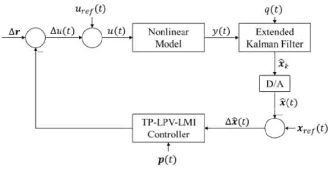
Figure 2. Structure of the control loop.
C. Final Control Structure
We have considered the original model as reference model during the controller design by assuming that it is an exactly known model from parameter and dynamics point of view.
This model can be replaced by any arbitrary, but appropriate model, however.
The finalized control structure can be seen in Fig. 2. We have applied permanenturef(t) = uref = 14 [mg/kg/min]
which guaranteed that x1(t) = 1 [mm3] at the end of the therapy.
Since thex2andx3state variables of the controlled system cannot be measured we applied an Extended Kalman Filter (EKF) to estimate them. The EKF was a mixed continu- ous/discrete EKF with T = 1 day sampling time in its measurement part [17], [33].
Through the control framework the controller enforces the original model to behave as the given reference model, namely, x(t) = xref(t), t → ∞. This is equivalent to Δr = x− xref = 0, where Δr =0, namely, the controller eliminates the deviation betweenxandxref over time.
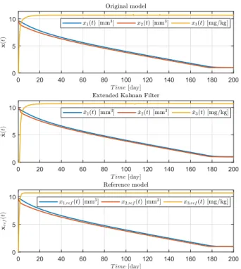
IV. RESULTS
The validation of the developed control en- vironment have been realized in the MATLAB Simulink environment. The applied initial conditions have been x(t0) = [ln(14900),ln(14900),0], xref(t0) = [ln(17000), ln(17000),0], x(tˆ 0) = [ln(17000), ln(17000),0], respectively. The initial conditions were arbitrarily selected, however, we assumed the lack of therapeutic agents before the beginning of the therapy (x3(t0) = ˆx3(t0) =xref,3(t0) = 0) and thexref(t0) = ˆx(t0), thus the reference and EKF state variables are adjusted by us at the beginning of the therapy. The selected values were reasonable from the viewpoint of the domain ofxi.
We have not considered noises and disturbances in this study in accordance with the properties of the model, i.e.d≡0and n≡ 0. This assumption leaded the EKF to be acting as an optimal estimator [33].
Figure 3 presents the state trajectories of the original system (x(t)), the EKF (ˆx(t)) and the reference system xref(t),
Figure 3. Trajectories of the state variables:x(t)original system,ˆx(t)EKF, xref(t)reference system.
respectively. It can be seen that both of them are quite similar.
The controlled system and the EKF are approaching the reference model with high accuracy. The final values forx1 andx2in the case of all models are1mm3which is the lower boundary of the domain of the states as it was expected.
Figure 4 shows the deviation between the state variables of the different systems. The upper subfigure is the difference between the original system and the EKF, namely,x(t)−x(t).ˆ In the closed-loop the EKF approximates the states of the original system. It can be seen that this approximation is loaded with small error in the case ofx1andx2compared to the magnitudes of the states, further, this small error decays fast as well. The higher, but quickly decaying error inx3(t) is coming from the discretization error. The middle subfigure is the difference between the reference system and the EKF, that isxref(t)−ˆx(t). From the controller point of view, this is the important aspect, since this is the error signal to be considered by the controller. The same phenomena occurs as in the previous case, namely, the initial errors decay rapidly. The lower subfigure represents the difference between the reference system and the original system, namely,xref(t)−x(t). The figure shows that the deviations are small, moreover, rapidly decay. The final Root Mean Square Error (RMSE) for all state variables are the following over the whole time domain:
• RMSEx(t)−ˆx(t) = [2.2290,3.8269,3.5293];
• RMSExref(t)−ˆx(t)= [2.2116,3.8149,5.4068];
• RMSExref(t)−x(t)= [0.1843,0.0565,2.0559].
Consequently, the controller operated well and enforced the
controlled original nonlinear system to be behave as the reference system.
Figure 4. Deviations between the states of the models.
Figure 5. The reference and realized control signals.
Figure 5 shows the reference uref(t) and control u(t)
signals, respectively. Due to the initial value discrepancy there was a higher peak-like difference between the uref(t) and u(t) which stabilized rapidly. There are different downward peaks in the u(t) around days 2,106 and 131 which are caused by the switches in the scheduling parameters. The uref was permanent 14 mg/kg/day as we mentioned already.
The RMSE based deviation between uref(t) and u(t) was 9.3994 over the whole simulated time horizon. The lower subfigure shows that the controller was able to keep the control signal on similar level as the reference signal, thus the control framework operated well from this point of view as well.
The totally injected reference inhibitor was Uref = 18298 [mg/kg], while the totally injected inhibitor was U = 18098 [mg/kg] which is only 200 [mg/kg] discrepancy.
V. CONCLUSION
In this study we have presented our latest developments regrading the control of tumor growth through anti-angiogenic treatment. We have applied the extended, transformed version of well-known Hahnfeldt-model from which two internal states have been estimated by EKF.
We have developed a difference based qLPV model which has been used via the LMI based controller design. The real- ization was done by applying the TP model transformation to generate TP controller. The resulting TP-LPV-LMI controller is able to provide stable control action in Lyapunov sense. We have found that the developed control framework operated well and it was able to enforce the controlled model to behave as the determined reference model.
In our future work we will develop more sophisticated reference model and embed the disturbance and noise effects to examine whether the controller can tolerates them or not.
ACKNOWLEDGMENT
The Authors thankfully acknowledge the support of the Robotics Special College of ´Obuda University and the ´Obuda University’s Research, Innovation and Service Center.
REFERENCES
[1] N. Vasudev and A. Reynolds, “Anti-angiogenic therapy for cancer: cur- rent progress, unresolved questions and future directions,”Angiogenesis, vol. 17, no. 3, pp. 471–494, 2014.
[2] P. Charlton and J. Spicer, “Targeted therapy in cancer,”Medicine, vol. 44, no. 1, pp. 34–38, 2016.
[3] R. Weinberg,The biology of cancer, 2nd ed. New York, USA: Garland Science, Taylor and Francis, 2014.
[4] A. M. Abdalla, L. Xiao, M. W. Ullah, M. Yu, C. Ouyang, and G. Yang,
“Current challenges of cancer anti-angiogenic therapy and the promise of nanotherapeutics,”Theranostics, vol. 8, no. 2, pp. 533–548, 2018.
[5] J. S´api, L. Kov´acs, D. Drexler, P. Kocsis, D. Ga´ari, and Z. S´api,
“Tumor volume estimation and quasi-continuous administration for most effective bevacizumab therapy,”PLoS ONE, vol. 10, no. 11, 2015.
[6] D. Drexler, J. S´api, and L. Kov´acs, “Potential Benefits of Discrete-Time Controller-based Treatments over Protocol-based Cancer Therapies,”
ACTA Pol Hung, vol. 14, no. 1, pp. 11–23, 2017.
[7] J. S´api, “Controller-managed automated therapy and tumor growth model identification in the case of antiangiogenic therapy for most ef- fective, individualized treatment,” Ph.D. dissertation, ´Obuda University, Budapest, Hungary, 2015.
[8] D. A. Drexler, J. S´api, and L. Kov´acs, “Positive nonlinear control of tumor growth using angiogenic inhibition,”IFAC-PapersOnLine, vol. 50, no. 1, pp. 15 068 – 15 073, 2017, 20th IFAC World Congress.
[9] A. White, G. Zhu, and J. Choi,Linear Parameter Varying Control for Engineering Applicaitons, 1st ed. London: Springer, 2013.
[10] L. Kov´acs, “Linear parameter varying (LPV) based robust control of type-I diabetes driven for real patient data,”Knowl-Based Syst, vol. 122, pp. 199–213, 2017.
[11] S. Boyd, L. El Ghaoui, E. Feron, and V. Balakrishnan,Linear Matrix Inequalities in System and Control Theory, ser. Studies in Applied Mathematics. Philadelphia, PA: SIAM, 1994, vol. 15.
[12] G. Herrmann, M. C. Turner, and I. Postlethwaite, “Linear matrix in- equalities in control,” inMathematical methods for robust and nonlinear control. Springer, 2007, pp. 123–142.
[13] P. Baranyi, Y. Yam, and P. Varlaki, Tensor Product Model Transfor- mation in Polytopic Model-Based Control, 1st ed. USA: CRC Press, 2013.
[14] R.-E. Precup, R.-C. David, and E. M. Petriu, “Grey wolf optimizer algorithm-based tuning of fuzzy control systems with reduced parametric sensitivity,”IEEE Transactions on Industrial Electronics, vol. 64, no. 1, pp. 527–534, 2017.
[15] P. Baranyi, “Extension of the Multi-TP Model Transformation to Func- tions with Different Numbers of Variables,”Complexity, vol. 2018, 2018.
[16] D. Copot, R. De Keyser, J. Juchem, and C. Ionescu, “Fractional order impedance model to estimate glucose concentration: in vitro analysis,”
ACTA Pol Hung, vol. 14, no. 1, pp. 207–220, 2017.
[17] M. Grewal and A. Andrews, Kalman Filtering: Theory and Practice Using MATLAB, 3rd ed. Chichester, UK: John Wiley and Sons, 2008.
[18] P. Hahnfeldt, D. Panigrahy, J. Folkman, and L. Hlatky, “Tumor develop- ment under angiogenic signaling: A dynamical theory of tumor growth, treatment response, and postvascular dormancy,”Cancer Res, vol. 59, pp. 4770–4775, 1999.
[19] J. Klamka, H. Maurer, and A. Swierniak, “Local controllability and optimal control for amodel of combined anticancer therapy with control delays,”Math Biosci Eng, vol. 14, no. 1, pp. 195–216, 2017.
[20] J. S´api, D. A. Drexler, and L. Kov´acs, “Potential Benefits of Discrete- Time Controllerbased Treatments over Protocol-based Cancer Thera- pies,”Acta Pol Hung, vol. 14, no. 1, pp. 11–23, 2017.
[21] J. Mohammadpour and C. W. Scherer,Control of linear parameter varying systems with applications. Springer Science & Business Media, 2012.
[22] J. Kuti, P. Galambos, and P. Baranyi, “Control analysis and synthesis through polytopic tensor product model: a general concept,” IFAC- PapersOnLine, vol. 50, no. 1, pp. 6558–6563, 2017.
[23] G. B. Thomas, R. L. Finney, M. D. Weir, and F. R. Giordano,Thomas’
calculus. Addison-Wesley Reading, 2003.
[24] J. Kuti, P. Galambos, and P. Baranyi, “Minimal volume simplex (MVS) convex hull generation and manipulation methodology for TP model transformation,”Asian J Control, vol. 19, no. 1, pp. 289–301, 2017.
[25] ——, “Generalization of tensor product model transformation for control design,”IFAC-PapersOnLine, vol. 50, no. 1, pp. 5604–5609, 2017.
[26] A. Szollosi and P. Baranyi, “Influence of the Tensor Product Model Representation of qLPV Models on the Feasibility of Linear Matrix Inequality Based Stability Analysis,”Asian J Control, vol. 20, no. 1, pp. 531–547, 2018.
[27] X. Liu, Y. Yu, Z. Li, H. H. Iu, and T. Fernando, “An Efficient Algorithm for Optimally Reshaping the TP Model Transformation,”
IEEE T Circuits-II, vol. 64, no. 10, pp. 1187–1191, 2017.
[28] P. G. M. Chilali and P. Apkarian, “Robust Pole Placement in LMI Regions,”IEEE T Automat Contr, vol. 44, no. 12, pp. 2257 – 2270, 1999.
[29] M. Chilali and P. Gahinet, “H∞ Design with Pole Placement Con- straints: An LMI Approach,” IEEE Transactions on Automatic Control,”
IEEE T Automat Contr, vol. 41, no. 3, pp. 358 – 367, 1996.
[30] K. Tanaka and H. O. Wang,Fuzzy Control Systems Design and Analysis:
A Linear Matrix Inequality Approach, 1st ed. Chichester, UK: John Wiley and Sons, 2001.
[31] J. L¨ofberg, “Yalmip : A toolbox for modeling and optimization in matlab,” in Proceedings of the CACSD Conference, Taipei, Taiwan, 2004.
[32] I. Polik, T. Terlaky, and Y. Zinchenko, “Sedumi: a package for conic optimization,” inIMA workshop on Optimization and Control, Univ.
Minnesota, Minneapolis. Citeseer, 2007.
[33] H. Musoff and P. Zarchan, Fundamentals of Kalman Filtering: A Practical Approach, 3rd ed. American Institute of Aeronautics and Astronautics, 2009.