Road surface estimation based LPV control design for autonomous

IFAC PapersOnLine 52-28 (2019) 120–125

ScienceDirect

2405-8963 © 2019, IFAC (International Federation of Automatic Control) Hosting by Elsevier Ltd. All rights reserved.

Peer review under responsibility of International Federation of Automatic Control.

10.1016/j.ifacol.2019.12.358

© 2019, IFAC (International Federation of Automatic Control) Hosting by Elsevier Ltd. All rights reserved.

10.1016/j.ifacol.2019.12.358 2405-8963

Road surface estimation based LPV control design for autonomous

vehicles

D´aniel F´enyes,Bal´azs N´emeth,P´eter G´asp´ar, Zolt´an Szab´o Systems and Control Laboratory, Institute for Computer Science and

Control, Hungarian Academy of Sciences, Budapest, Hungary;

E-mail:

[daniel.fenyes,balazs.nemeth,peter.gaspar,zoltan.szabo]@sztaki.mta.hu

Abstract:The paper proposes a new road surface estimation algorithm for autonomous vehicles using a machine-learning based method, which is in cooperation with the lateral control of the vehicle. The algorithm uses large datasets, which can be collected e.g. from the on-board sensors of the vehicle, or it also can be provided by vehicle dynamic simulation softwares. The result of the surface estimation is built-in the lateral control system as a scheduling parameter.

Furthermore, the lateral control design is based on the Linear Parameter Varying (LPV) method, which guarantees the safe motion of the vehicle against varying parameters of the system. Finally, a comprehensive simulation is presented to show the efficiency and the operation of the proposed control system.

Keywords: road surface estimation, big data analysis, autonomous vehicle systems 1. INTRODUCTION AND MOTIVATION

In the last few years, the automotive companies have shifted their focal towards the development of the highly- automated, autonomous vehicles. This new trend has brought numerous challenges for the automotive industry.

One of these challenges is the design of the optimal, robust controllers, which are able to maintain the required perfor- mances under various circumstances. This means that the autonomous vehicles have to be able to work on different roads and even under extreme weather conditions. This capability of the control system involves several measure- ments and estimations in order to appropriately adjust itself to the actual driving-situation. Therefore, the accu- racy of the estimation of the adhesion coefficient between the tire and the road crucially influences the operation of the autonomous vehicle.

Over the past few decades, several methods have been developed for the estimation problem of road surfaces.

These solutions can be divided into three main categories:

1. Camera and vision-based methods, 2. Model-based approaches, 3. Machine-learning based algorithms. In the followings these methods are revised briefly.

This work has been supported by the grant ’2018-1.2.1-NKP- 00008: Exploring the Mathematical Foundations of Artificial Intelli- gence’. The work of Bal´azs N´emeth was partially supported by the J´anos Bolyai Research Scholarship of the Hungarian Academy of Sciences and the ´UNKP-19-4 New National Excellence Program of the Ministry for Innovation and Technology. The work of D´aniel F´enyes was partially supported by the ´UNKP-19-3 New National Excellence Program of the Ministry for Innovation and Technology.

Camera and vision-based approaches use the images of the on-board camera to estimate the road surface and the adhesion coefficient. Islam et al. [2018] presents a method to classify different road surfaces using the RGB channels and their intensity histograms, whose accuracy is around 78.6%. Sun and Jia [2018] combines the camera-based and the machine learning approaches. It presents several machine learning algorithm such as: K-NN, Neural Net- work and SVM and naive-Bayesian SVM, which classify the road surface using the image of the on-board camera.

They conclude that the best results is given by the naive- Bayesian SVM algorithm.

Another group of the estimation methods is the model- based estimators. For example, M¨uller et al. [2003] de- scribes a method to estimate the adhesion coefficient using the slip of the vehicle. The accuracy of this solution is close to 80%. Another model-based estimator is presented in Rath et al. [2013]. This approach uses a simple quarter car and the LuGre friction models to estimate the actual µvalue.

The last group includes the machine-learning and deep- learning based solutions. In the past few decades, the passenger cars have been equipped with a lot of sensors such as accelerometers, gyroscopes, GPS etc. These sensors are used for different purposes. For example: ABS, ASR, ESP systems. Although these systems use only the current measurements of the devices, the information, which is provided by them, can be collected and stored on an in- ternal, or a cloud-based memory. A SVM (Support vector machine) based solution is presented in Li et al. [2012].

Road surface estimation based LPV control design for autonomous

vehicles

D´aniel F´enyes,Bal´azs N´emeth,P´eter G´asp´ar, Zolt´an Szab´o Systems and Control Laboratory, Institute for Computer Science and

Control, Hungarian Academy of Sciences, Budapest, Hungary;

E-mail:

[daniel.fenyes,balazs.nemeth,peter.gaspar,zoltan.szabo]@sztaki.mta.hu

Abstract:The paper proposes a new road surface estimation algorithm for autonomous vehicles using a machine-learning based method, which is in cooperation with the lateral control of the vehicle. The algorithm uses large datasets, which can be collected e.g. from the on-board sensors of the vehicle, or it also can be provided by vehicle dynamic simulation softwares. The result of the surface estimation is built-in the lateral control system as a scheduling parameter.

Furthermore, the lateral control design is based on the Linear Parameter Varying (LPV) method, which guarantees the safe motion of the vehicle against varying parameters of the system. Finally, a comprehensive simulation is presented to show the efficiency and the operation of the proposed control system.

Keywords: road surface estimation, big data analysis, autonomous vehicle systems 1. INTRODUCTION AND MOTIVATION

In the last few years, the automotive companies have shifted their focal towards the development of the highly- automated, autonomous vehicles. This new trend has brought numerous challenges for the automotive industry.

One of these challenges is the design of the optimal, robust controllers, which are able to maintain the required perfor- mances under various circumstances. This means that the autonomous vehicles have to be able to work on different roads and even under extreme weather conditions. This capability of the control system involves several measure- ments and estimations in order to appropriately adjust itself to the actual driving-situation. Therefore, the accu- racy of the estimation of the adhesion coefficient between the tire and the road crucially influences the operation of the autonomous vehicle.

Over the past few decades, several methods have been developed for the estimation problem of road surfaces.

These solutions can be divided into three main categories:

1. Camera and vision-based methods, 2. Model-based approaches, 3. Machine-learning based algorithms. In the followings these methods are revised briefly.

This work has been supported by the grant ’2018-1.2.1-NKP- 00008: Exploring the Mathematical Foundations of Artificial Intelli- gence’. The work of Bal´azs N´emeth was partially supported by the J´anos Bolyai Research Scholarship of the Hungarian Academy of Sciences and the ´UNKP-19-4 New National Excellence Program of the Ministry for Innovation and Technology. The work of D´aniel F´enyes was partially supported by the ´UNKP-19-3 New National Excellence Program of the Ministry for Innovation and Technology.

Camera and vision-based approaches use the images of the on-board camera to estimate the road surface and the adhesion coefficient. Islam et al. [2018] presents a method to classify different road surfaces using the RGB channels and their intensity histograms, whose accuracy is around 78.6%. Sun and Jia [2018] combines the camera-based and the machine learning approaches. It presents several machine learning algorithm such as: K-NN, Neural Net- work and SVM and naive-Bayesian SVM, which classify the road surface using the image of the on-board camera.

They conclude that the best results is given by the naive- Bayesian SVM algorithm.

Another group of the estimation methods is the model- based estimators. For example, M¨uller et al. [2003] de- scribes a method to estimate the adhesion coefficient using the slip of the vehicle. The accuracy of this solution is close to 80%. Another model-based estimator is presented in Rath et al. [2013]. This approach uses a simple quarter car and the LuGre friction models to estimate the actual µvalue.

The last group includes the machine-learning and deep- learning based solutions. In the past few decades, the passenger cars have been equipped with a lot of sensors such as accelerometers, gyroscopes, GPS etc. These sensors are used for different purposes. For example: ABS, ASR, ESP systems. Although these systems use only the current measurements of the devices, the information, which is provided by them, can be collected and stored on an in- ternal, or a cloud-based memory. A SVM (Support vector machine) based solution is presented in Li et al. [2012].

Road surface estimation based LPV control design for autonomous

vehicles

D´aniel F´enyes,Bal´azs N´emeth,P´eter G´asp´ar, Zolt´an Szab´o Systems and Control Laboratory, Institute for Computer Science and

Control, Hungarian Academy of Sciences, Budapest, Hungary;

E-mail:

[daniel.fenyes,balazs.nemeth,peter.gaspar,zoltan.szabo]@sztaki.mta.hu

Abstract:The paper proposes a new road surface estimation algorithm for autonomous vehicles using a machine-learning based method, which is in cooperation with the lateral control of the vehicle. The algorithm uses large datasets, which can be collected e.g. from the on-board sensors of the vehicle, or it also can be provided by vehicle dynamic simulation softwares. The result of the surface estimation is built-in the lateral control system as a scheduling parameter.

Furthermore, the lateral control design is based on the Linear Parameter Varying (LPV) method, which guarantees the safe motion of the vehicle against varying parameters of the system. Finally, a comprehensive simulation is presented to show the efficiency and the operation of the proposed control system.

Keywords: road surface estimation, big data analysis, autonomous vehicle systems 1. INTRODUCTION AND MOTIVATION

In the last few years, the automotive companies have shifted their focal towards the development of the highly- automated, autonomous vehicles. This new trend has brought numerous challenges for the automotive industry.

One of these challenges is the design of the optimal, robust controllers, which are able to maintain the required perfor- mances under various circumstances. This means that the autonomous vehicles have to be able to work on different roads and even under extreme weather conditions. This capability of the control system involves several measure- ments and estimations in order to appropriately adjust itself to the actual driving-situation. Therefore, the accu- racy of the estimation of the adhesion coefficient between the tire and the road crucially influences the operation of the autonomous vehicle.

Over the past few decades, several methods have been developed for the estimation problem of road surfaces.

These solutions can be divided into three main categories:

1. Camera and vision-based methods, 2. Model-based approaches, 3. Machine-learning based algorithms. In the followings these methods are revised briefly.

This work has been supported by the grant ’2018-1.2.1-NKP- 00008: Exploring the Mathematical Foundations of Artificial Intelli- gence’. The work of Bal´azs N´emeth was partially supported by the J´anos Bolyai Research Scholarship of the Hungarian Academy of Sciences and the ´UNKP-19-4 New National Excellence Program of the Ministry for Innovation and Technology. The work of D´aniel F´enyes was partially supported by the ´UNKP-19-3 New National Excellence Program of the Ministry for Innovation and Technology.

Camera and vision-based approaches use the images of the on-board camera to estimate the road surface and the adhesion coefficient. Islam et al. [2018] presents a method to classify different road surfaces using the RGB channels and their intensity histograms, whose accuracy is around 78.6%. Sun and Jia [2018] combines the camera-based and the machine learning approaches. It presents several machine learning algorithm such as: K-NN, Neural Net- work and SVM and naive-Bayesian SVM, which classify the road surface using the image of the on-board camera.

They conclude that the best results is given by the naive- Bayesian SVM algorithm.

Another group of the estimation methods is the model- based estimators. For example, M¨uller et al. [2003] de- scribes a method to estimate the adhesion coefficient using the slip of the vehicle. The accuracy of this solution is close to 80%. Another model-based estimator is presented in Rath et al. [2013]. This approach uses a simple quarter car and the LuGre friction models to estimate the actual µvalue.

The last group includes the machine-learning and deep- learning based solutions. In the past few decades, the passenger cars have been equipped with a lot of sensors such as accelerometers, gyroscopes, GPS etc. These sensors are used for different purposes. For example: ABS, ASR, ESP systems. Although these systems use only the current measurements of the devices, the information, which is provided by them, can be collected and stored on an in- ternal, or a cloud-based memory. A SVM (Support vector machine) based solution is presented in Li et al. [2012].

Road surface estimation based LPV control design for autonomous

vehicles

D´aniel F´enyes,Bal´azs N´emeth,P´eter G´asp´ar, Zolt´an Szab´o Systems and Control Laboratory, Institute for Computer Science and

Control, Hungarian Academy of Sciences, Budapest, Hungary;

E-mail:

[daniel.fenyes,balazs.nemeth,peter.gaspar,zoltan.szabo]@sztaki.mta.hu

Abstract:The paper proposes a new road surface estimation algorithm for autonomous vehicles using a machine-learning based method, which is in cooperation with the lateral control of the vehicle. The algorithm uses large datasets, which can be collected e.g. from the on-board sensors of the vehicle, or it also can be provided by vehicle dynamic simulation softwares. The result of the surface estimation is built-in the lateral control system as a scheduling parameter.

Furthermore, the lateral control design is based on the Linear Parameter Varying (LPV) method, which guarantees the safe motion of the vehicle against varying parameters of the system. Finally, a comprehensive simulation is presented to show the efficiency and the operation of the proposed control system.

Keywords: road surface estimation, big data analysis, autonomous vehicle systems 1. INTRODUCTION AND MOTIVATION

In the last few years, the automotive companies have shifted their focal towards the development of the highly- automated, autonomous vehicles. This new trend has brought numerous challenges for the automotive industry.

One of these challenges is the design of the optimal, robust controllers, which are able to maintain the required perfor- mances under various circumstances. This means that the autonomous vehicles have to be able to work on different roads and even under extreme weather conditions. This capability of the control system involves several measure- ments and estimations in order to appropriately adjust itself to the actual driving-situation. Therefore, the accu- racy of the estimation of the adhesion coefficient between the tire and the road crucially influences the operation of the autonomous vehicle.

Over the past few decades, several methods have been developed for the estimation problem of road surfaces.

These solutions can be divided into three main categories:

1. Camera and vision-based methods, 2. Model-based approaches, 3. Machine-learning based algorithms. In the followings these methods are revised briefly.

This work has been supported by the grant ’2018-1.2.1-NKP- 00008: Exploring the Mathematical Foundations of Artificial Intelli- gence’. The work of Bal´azs N´emeth was partially supported by the J´anos Bolyai Research Scholarship of the Hungarian Academy of Sciences and the ´UNKP-19-4 New National Excellence Program of the Ministry for Innovation and Technology. The work of D´aniel F´enyes was partially supported by the ´UNKP-19-3 New National Excellence Program of the Ministry for Innovation and Technology.

Camera and vision-based approaches use the images of the on-board camera to estimate the road surface and the adhesion coefficient. Islam et al. [2018] presents a method to classify different road surfaces using the RGB channels and their intensity histograms, whose accuracy is around 78.6%. Sun and Jia [2018] combines the camera-based and the machine learning approaches. It presents several machine learning algorithm such as: K-NN, Neural Net- work and SVM and naive-Bayesian SVM, which classify the road surface using the image of the on-board camera.

They conclude that the best results is given by the naive- Bayesian SVM algorithm.

Another group of the estimation methods is the model- based estimators. For example, M¨uller et al. [2003] de- scribes a method to estimate the adhesion coefficient using the slip of the vehicle. The accuracy of this solution is close to 80%. Another model-based estimator is presented in Rath et al. [2013]. This approach uses a simple quarter car and the LuGre friction models to estimate the actual µvalue.

The last group includes the machine-learning and deep- learning based solutions. In the past few decades, the passenger cars have been equipped with a lot of sensors such as accelerometers, gyroscopes, GPS etc. These sensors are used for different purposes. For example: ABS, ASR, ESP systems. Although these systems use only the current measurements of the devices, the information, which is provided by them, can be collected and stored on an in- ternal, or a cloud-based memory. A SVM (Support vector machine) based solution is presented in Li et al. [2012].

Road surface estimation based LPV control design for autonomous

vehicles

D´aniel F´enyes,Bal´azs N´emeth,P´eter G´asp´ar, Zolt´an Szab´o Systems and Control Laboratory, Institute for Computer Science and

Control, Hungarian Academy of Sciences, Budapest, Hungary;

E-mail:

[daniel.fenyes,balazs.nemeth,peter.gaspar,zoltan.szabo]@sztaki.mta.hu

Abstract:The paper proposes a new road surface estimation algorithm for autonomous vehicles using a machine-learning based method, which is in cooperation with the lateral control of the vehicle. The algorithm uses large datasets, which can be collected e.g. from the on-board sensors of the vehicle, or it also can be provided by vehicle dynamic simulation softwares. The result of the surface estimation is built-in the lateral control system as a scheduling parameter.

Furthermore, the lateral control design is based on the Linear Parameter Varying (LPV) method, which guarantees the safe motion of the vehicle against varying parameters of the system. Finally, a comprehensive simulation is presented to show the efficiency and the operation of the proposed control system.

Keywords: road surface estimation, big data analysis, autonomous vehicle systems 1. INTRODUCTION AND MOTIVATION

In the last few years, the automotive companies have shifted their focal towards the development of the highly- automated, autonomous vehicles. This new trend has brought numerous challenges for the automotive industry.

One of these challenges is the design of the optimal, robust controllers, which are able to maintain the required perfor- mances under various circumstances. This means that the autonomous vehicles have to be able to work on different roads and even under extreme weather conditions. This capability of the control system involves several measure- ments and estimations in order to appropriately adjust itself to the actual driving-situation. Therefore, the accu- racy of the estimation of the adhesion coefficient between the tire and the road crucially influences the operation of the autonomous vehicle.

Over the past few decades, several methods have been developed for the estimation problem of road surfaces.

These solutions can be divided into three main categories:

1. Camera and vision-based methods, 2. Model-based approaches, 3. Machine-learning based algorithms. In the followings these methods are revised briefly.

This work has been supported by the grant ’2018-1.2.1-NKP- 00008: Exploring the Mathematical Foundations of Artificial Intelli- gence’. The work of Bal´azs N´emeth was partially supported by the J´anos Bolyai Research Scholarship of the Hungarian Academy of Sciences and the ´UNKP-19-4 New National Excellence Program of the Ministry for Innovation and Technology. The work of D´aniel F´enyes was partially supported by the ´UNKP-19-3 New National Excellence Program of the Ministry for Innovation and Technology.

Camera and vision-based approaches use the images of the on-board camera to estimate the road surface and the adhesion coefficient. Islam et al. [2018] presents a method to classify different road surfaces using the RGB channels and their intensity histograms, whose accuracy is around 78.6%. Sun and Jia [2018] combines the camera-based and the machine learning approaches. It presents several machine learning algorithm such as: K-NN, Neural Net- work and SVM and naive-Bayesian SVM, which classify the road surface using the image of the on-board camera.

They conclude that the best results is given by the naive- Bayesian SVM algorithm.

Another group of the estimation methods is the model- based estimators. For example, M¨uller et al. [2003] de- scribes a method to estimate the adhesion coefficient using the slip of the vehicle. The accuracy of this solution is close to 80%. Another model-based estimator is presented in Rath et al. [2013]. This approach uses a simple quarter car and the LuGre friction models to estimate the actual µvalue.

The last group includes the machine-learning and deep- learning based solutions. In the past few decades, the passenger cars have been equipped with a lot of sensors such as accelerometers, gyroscopes, GPS etc. These sensors are used for different purposes. For example: ABS, ASR, ESP systems. Although these systems use only the current measurements of the devices, the information, which is provided by them, can be collected and stored on an in- ternal, or a cloud-based memory. A SVM (Support vector machine) based solution is presented in Li et al. [2012].

Road surface estimation based LPV control design for autonomous

vehicles

D´aniel F´enyes,Bal´azs N´emeth,P´eter G´asp´ar, Zolt´an Szab´o Systems and Control Laboratory, Institute for Computer Science and

Control, Hungarian Academy of Sciences, Budapest, Hungary;

E-mail:

[daniel.fenyes,balazs.nemeth,peter.gaspar,zoltan.szabo]@sztaki.mta.hu

Abstract:The paper proposes a new road surface estimation algorithm for autonomous vehicles using a machine-learning based method, which is in cooperation with the lateral control of the vehicle. The algorithm uses large datasets, which can be collected e.g. from the on-board sensors of the vehicle, or it also can be provided by vehicle dynamic simulation softwares. The result of the surface estimation is built-in the lateral control system as a scheduling parameter.

Furthermore, the lateral control design is based on the Linear Parameter Varying (LPV) method, which guarantees the safe motion of the vehicle against varying parameters of the system. Finally, a comprehensive simulation is presented to show the efficiency and the operation of the proposed control system.

Keywords: road surface estimation, big data analysis, autonomous vehicle systems 1. INTRODUCTION AND MOTIVATION

In the last few years, the automotive companies have shifted their focal towards the development of the highly- automated, autonomous vehicles. This new trend has brought numerous challenges for the automotive industry.

One of these challenges is the design of the optimal, robust controllers, which are able to maintain the required perfor- mances under various circumstances. This means that the autonomous vehicles have to be able to work on different roads and even under extreme weather conditions. This capability of the control system involves several measure- ments and estimations in order to appropriately adjust itself to the actual driving-situation. Therefore, the accu- racy of the estimation of the adhesion coefficient between the tire and the road crucially influences the operation of the autonomous vehicle.

Over the past few decades, several methods have been developed for the estimation problem of road surfaces.

These solutions can be divided into three main categories:

1. Camera and vision-based methods, 2. Model-based approaches, 3. Machine-learning based algorithms. In the followings these methods are revised briefly.

This work has been supported by the grant ’2018-1.2.1-NKP- 00008: Exploring the Mathematical Foundations of Artificial Intelli- gence’. The work of Bal´azs N´emeth was partially supported by the J´anos Bolyai Research Scholarship of the Hungarian Academy of Sciences and the ´UNKP-19-4 New National Excellence Program of the Ministry for Innovation and Technology. The work of D´aniel F´enyes was partially supported by the ´UNKP-19-3 New National Excellence Program of the Ministry for Innovation and Technology.

Camera and vision-based approaches use the images of the on-board camera to estimate the road surface and the adhesion coefficient. Islam et al. [2018] presents a method to classify different road surfaces using the RGB channels and their intensity histograms, whose accuracy is around 78.6%. Sun and Jia [2018] combines the camera-based and the machine learning approaches. It presents several machine learning algorithm such as: K-NN, Neural Net- work and SVM and naive-Bayesian SVM, which classify the road surface using the image of the on-board camera.

They conclude that the best results is given by the naive- Bayesian SVM algorithm.

Another group of the estimation methods is the model- based estimators. For example, M¨uller et al. [2003] de- scribes a method to estimate the adhesion coefficient using the slip of the vehicle. The accuracy of this solution is close to 80%. Another model-based estimator is presented in Rath et al. [2013]. This approach uses a simple quarter car and the LuGre friction models to estimate the actual µvalue.

The last group includes the machine-learning and deep- learning based solutions. In the past few decades, the passenger cars have been equipped with a lot of sensors such as accelerometers, gyroscopes, GPS etc. These sensors are used for different purposes. For example: ABS, ASR, ESP systems. Although these systems use only the current measurements of the devices, the information, which is provided by them, can be collected and stored on an in- ternal, or a cloud-based memory. A SVM (Support vector machine) based solution is presented in Li et al. [2012].

This technique requires relatively large steering angle in order to accurately estimate the adhesion coefficient.

The datasets, which are created from the saved signals, can provide good bases for any machine/deep learning tech- niques. These algorithms can catch the hidden knowledge from the datasets, which can be used for other nontrivial problems. For example, in this case, the road surface / adhesion coefficient estimation problem can be solved by using these techniques. Song et al. [2017] describes a BP neural network-based technique, which is able to estimate the adhesion coefficient at constant velocity with relatively high accuracy.

One of the main contributions of the paper is a machine- learning based road surface estimation method, which uses only the available signals from the on-board system.

Since, the accurate estimation of the adhesion coefficient cannot not possible in all vehicle dynamic situation, the estimation solution classifies the road surface into three categories:dry∈ {0.7−1.0},wet∈ {0.4−0.7},icy∈ {0.0− 0.4}. As it can be seen, each category covers a predefined range of the adhesion coefficient from 0.0 up to 1.0. Asa further contribution, the result of the estimation has been built-in in the lateral control design, which is based on the LPV (Linear Parameter Varying) method, in which the estimate of the road surface is used as a scheduling parameter.

The paper follows the following structure: In the next section, the acquisition of the collected data is presented.

Third section presents the machine-learning algorithm and its application in the lateral control design. The LPV- based control design is detailed in the fourth section. Fi- nally, a comprehensive illustration of the proposed control system is given in the last section.

2. DATA ACQUISITION AND BIG DATA ANALYSIS As all machine-learning algorithms demand a lot of data to provide reliable results, the most significant step of this research is the data acquisition. In this paper, the large amount of data is provided by the high-fidelity simulation software, CarSim. In the simulation environment several simulations have been performed, in which some param- eters of the car and its environment were modified, such as longitudinal velocity of the vehicle and the adhesion coefficient between the tire and the road. Each value of the adhesion coefficient is associated with a distinctive road surface (icy, wet, dry). During the simulations several signals have been measured and collected: longitudinal acceleration, lateral acceleration, longitudinal velocity, lat- eral velocity, yaw rate, angular velocity of wheels, steering angle of front wheels, angle of steering wheel, side-slip angle of the vehicle, slip angles of the wheels, torques of the wheels, roll rate.

Since the goal of the estimation of the adhesion coefficient is to determine the peak value of this attribute, not in generalµ, the instances, in which the adhesion coefficient is close to its peak value must be found. For this purpose, several criteria can found in the literature e.g. in Li et al.

[2012]. It uses the values of yaw-rate, steering speed, lateral acceleration, longitudinal speed with some limitations to select the appropriate instances. However, in this paper, a

new criterion is used based on a stability condition, which was presented by Fenyes et al. [2018]. The original stability condition can be written as:

−ε < |1 +α1|

|1 +δ−β−^lv¹x^ψ˙|−1≤ε, (1) whereε is an experimentally defined parameter, l1 is the distance between the CG of the vehicle and the front axle andα1 is the mean value of the slips of the front wheels. The basic idea of this criterion relies on the deviation of the dynamical behaviors of the real vehicle and the linearized model. This deviation is large when the vehicle has high values of speed and steering angle, which indicates that the vehicle gets close to the peak value ofµ. Therefore, after some changes, this condition can be used as a selection criterion for the current case:

ε < |1 +α1|

|1 +δ−β−^lv¹x^ψ˙| −1 or |1 +α1|

|1 +δ−β−^lv¹x^ψ˙| −1<−ε, (2) In this case, the parameterεshould be as small as possible in order to not exclude too many instances.

2.1 Pace regression

There are a lot of machine-learning algorithms that can be used to estimate specific parameters/variables. Some of them yield complex models, which are hard to be used in online control system. Therefore, the so-called Pace Regression method is applied, which fits a simple linear model to the given problem. A brief introduction to this algorithm is given in this section, more detailed description can be found in Wang and Witten [1999]. Assume that the dataset consists of n independent instances, k measured variables and one output variable (the estimated variable). From the dataset, a matrixXcan be created.ζ^∗is a vector containing the parameters. Then, the output is determined as:

y=Xζ^∗+, (3)

where is the noise vector whose elements are sampled fromN(0, σ²).

It is also assumed thatσ² is known or, at least, it can be estimated (ˆσ²). M(ζ) denotes a fitted, linear model that has an unique parameter vectorζ while the true model is denoted byM(ζ^∗). The aim of the modeling task is to find a model from the entire model spaceM={M(ζ) :ζ∈R^k} whose predictive accuracy is the greatest on the given dataset.

3. ESTIMATION ALGORITHM

The whole control system, including the estimation al- gorithm, is divided into 5 parts: 1. Data collection, 2. Prepocess of data, 3. Regression, 4. Resulted model and 5. Control system. Each part is described briefly in this section:

This technique requires relatively large steering angle in order to accurately estimate the adhesion coefficient.

The datasets, which are created from the saved signals, can provide good bases for any machine/deep learning tech- niques. These algorithms can catch the hidden knowledge from the datasets, which can be used for other nontrivial problems. For example, in this case, the road surface / adhesion coefficient estimation problem can be solved by using these techniques. Song et al. [2017] describes a BP neural network-based technique, which is able to estimate the adhesion coefficient at constant velocity with relatively high accuracy.

One of the main contributions of the paper is a machine- learning based road surface estimation method, which uses only the available signals from the on-board system.

Since, the accurate estimation of the adhesion coefficient cannot not possible in all vehicle dynamic situation, the estimation solution classifies the road surface into three categories:dry∈ {0.7−1.0},wet∈ {0.4−0.7},icy∈ {0.0− 0.4}. As it can be seen, each category covers a predefined range of the adhesion coefficient from 0.0 up to 1.0. Asa further contribution, the result of the estimation has been built-in in the lateral control design, which is based on the LPV (Linear Parameter Varying) method, in which the estimate of the road surface is used as a scheduling parameter.

The paper follows the following structure: In the next section, the acquisition of the collected data is presented.

Third section presents the machine-learning algorithm and its application in the lateral control design. The LPV- based control design is detailed in the fourth section. Fi- nally, a comprehensive illustration of the proposed control system is given in the last section.

2. DATA ACQUISITION AND BIG DATA ANALYSIS As all machine-learning algorithms demand a lot of data to provide reliable results, the most significant step of this research is the data acquisition. In this paper, the large amount of data is provided by the high-fidelity simulation software, CarSim. In the simulation environment several simulations have been performed, in which some param- eters of the car and its environment were modified, such as longitudinal velocity of the vehicle and the adhesion coefficient between the tire and the road. Each value of the adhesion coefficient is associated with a distinctive road surface (icy, wet, dry). During the simulations several signals have been measured and collected: longitudinal acceleration, lateral acceleration, longitudinal velocity, lat- eral velocity, yaw rate, angular velocity of wheels, steering angle of front wheels, angle of steering wheel, side-slip angle of the vehicle, slip angles of the wheels, torques of the wheels, roll rate.

Since the goal of the estimation of the adhesion coefficient is to determine the peak value of this attribute, not in generalµ, the instances, in which the adhesion coefficient is close to its peak value must be found. For this purpose, several criteria can found in the literature e.g. in Li et al.

[2012]. It uses the values of yaw-rate, steering speed, lateral acceleration, longitudinal speed with some limitations to select the appropriate instances. However, in this paper, a

new criterion is used based on a stability condition, which was presented by Fenyes et al. [2018]. The original stability condition can be written as:

−ε < |1 +α1|

|1 +δ−β−^lv¹x^ψ˙|−1≤ε, (1) whereε is an experimentally defined parameter, l1 is the distance between the CG of the vehicle and the front axle andα1 is the mean value of the slips of the front wheels.

The basic idea of this criterion relies on the deviation of the dynamical behaviors of the real vehicle and the linearized model. This deviation is large when the vehicle has high values of speed and steering angle, which indicates that the vehicle gets close to the peak value of µ. Therefore, after some changes, this condition can be used as a selection criterion for the current case:

ε < |1 +α1|

|1 +δ−β−^lv¹x^ψ˙| −1 or |1 +α1|

|1 +δ−β−^lv¹x^ψ˙|−1<−ε, (2) In this case, the parameterεshould be as small as possible in order to not exclude too many instances.

2.1 Pace regression

There are a lot of machine-learning algorithms that can be used to estimate specific parameters/variables. Some of them yield complex models, which are hard to be used in online control system. Therefore, the so-called Pace Regression method is applied, which fits a simple linear model to the given problem. A brief introduction to this algorithm is given in this section, more detailed description can be found in Wang and Witten [1999]. Assume that the dataset consists of n independent instances, k measured variables and one output variable (the estimated variable).

From the dataset, a matrixXcan be created.ζ^∗is a vector containing the parameters. Then, the output is determined as:

y=Xζ^∗+, (3)

where is the noise vector whose elements are sampled fromN(0, σ²).

It is also assumed thatσ² is known or, at least, it can be estimated (ˆσ²). M(ζ) denotes a fitted, linear model that has an unique parameter vectorζ while the true model is denoted byM(ζ^∗). The aim of the modeling task is to find a model from the entire model spaceM={M(ζ) :ζ∈R^k} whose predictive accuracy is the greatest on the given dataset.

3. ESTIMATION ALGORITHM

The whole control system, including the estimation al- gorithm, is divided into 5 parts: 1. Data collection, 2.

Prepocess of data, 3. Regression, 4. Resulted model and 5. Control system. Each part is described briefly in this section:

Data collection: The acquisition and collection of data have been already presented in the Section 2. As men- tioned, the data is provided by the CarSim simulation software.

Prepocess: The prepocess step includes the data sepa- ration, which has been presented, and one more task: Since all of the measurements contains noises, the signals must be filtered before using them in the estimation. Therefore, all measured attributes are averaged over a time periodT:

Aˆi,t=

t

n=t−T

Ai,n

T (4)

whereAi,t is thet^thinstance ofi^th attribute.

Regression: The filtered and separated data is used in the regression step. As mentioned in the Section 2, all values of the adhesion coefficient is associated with a category of the road surface (icy, wet, dry). In this case, all road surface types are represented by their averaged adhesion coefficients. (dry: 0.85, wet: 0.55, icy: 0.2) The

Fig. 1. Result of the regression

results of the Pace Regression algorithm can be seen in Figure 3. The figure shows that the estimation algorithm is very good at separating the icy and wet cases. But it has a significant overlay at the wet and dry cases. Although this overlay is relatively large, it does not cause any dangerous situation. Moreover, in order to avoid fluctuation in the estimation, the numerical value ˆµ, which is provided by the estimation, is converted into the corresponding predefined categories (dry, wet, icy) in the following way:

round(10M(ˆµi))

10 ∈C(ˆµ) (5)

˜

µ=R(C(ˆµ)) (6)

where i = 1..n, n is an experimentally defined value, M gives the median value of a set and C(ˆµ) denotes the category (dry, wet, icy), which the given instance belongs to. Rgives the mean value of the category.

Finally, ˜µis used in the following.

Resulted model: The result of the Pace Regression algorithm can be used as a scheduling parameter in the LPV control design. All of the considered road surfaces is associated with a gridded model, which are used in the control design. Moreover, the yielded control system can select the best fitting controller using the road surface information. In this manner, the stability and the safe motion of the vehicle is guaranteed.

Control system: As mentioned, the control system uses the estimation of the road surface to calculate the optimal controller and the control input for the vehicle. The design of the lateral controller is presented in the next section.

4. LPV-BASED VEHICLE CONTROL DESIGN AND VELOCITY SELECTION STRATEGY

The goal of this section is to provide a control strategy, in which the design of the steering actuation is coordi- nated and the safe motion of the autonomous vehicle is guaranteed. The steering control design based on the LPV method is presented. It uses the result of the ˜µestimation through a scheduling variable.

Design of lateral LPV control

The design of the steering control is based on the formula- tion of the lateral dynamics in a linear model (Rajamani [2005])

mvx( ˙ψ+ ˙β) =Fy(α1) +Fy(α2), (7a) Jψ¨=Fy(α1)l1−Fy(α2)l2, (7b)

˙

vy =vx( ˙ψ+ ˙β), (7c) where m is the vehicle mass, J is the yaw-inertia and α1=δ−β−ψl˙ 1/vx,α2=β+ ˙ψl2/vx. As an assumption in the vehicle control problems, the lateral tire force Fy

is approximated in a linear form, such asFy =Cα. The representation of (7) is transformed into the parameter- varying state-space model

˙

x=A(ρ)x+B(ρ1)u, (8) where the state vector is x = ψ β v˙ y y^T

, the control input isu=δandρ=µis the selected scheduling variable of the system. Moreover,A(ρ),B(ρ) are matrices of system (8).

The goal of the control design is to guarantee the requested motion of the vehicle with minimum steering control in- tervention. Thus, the following performances are specified.

• Minimization of the lateral error The designed con- trol must reduce the error between the lateral position of the vehicley and the reference pathyref:

z1=yref −y, |z1| →min. (9)

• Minimization of the yaw-rate errorThe improvement of the path tracking requires the consideration of the turning motion of the vehicle through the yaw-rate, such as

z2= ˙ψref −ψ,˙ |z2| →min, (10) where ˙ψref represents the reference yaw-rate of the vehicle, which depends on the longitudinal velocity Rajamani [2005].

• Minimization of the actuation The path tracking of the vehicle must be guaranteed through minimum steering intervention, which leads to the performance z3=δ, |z3| →min. (11) The specified performances are compressed into a vector z= [z1 z2 z3]^T, which leads to the performance equation

z=C1x+D11r+D12u, (12) whereC1, D11, D12are matrices andrcontains the signals yref and ˙ψref.

The design of the LPV control requires the system dy- namics in the state-space form (8) and the performance equation (12). Moreover, it is necessary to scale the input and output signals of the plant, as it is illustrated in Figure 2. In practice, the scaling of the signals during the design process is performed through transfer functions G´asp´ar et al. [2017]. The role of Wref,1, Wref,2 is to scale the signals yref, ˙ψref. Similarly, Ww,1, Ww,2 scale the noises on the lateral position and on the yaw-rate measure- ments. Noises wy and wψ˙ are incorporated in the vector w=r wy wψ˙

^T

. The priority among the performances is guaranteed byWref,i,i={1,2,3}. The transfer functions Wref,i, i = {1,2} are selected in a second-order form to reach the smooth tracking of the reference signals. How- ever, in case of Wref,3 a first-order proportional transfer function can be enough to guarantee the minimization of δ.

P(ρ)

K(ρ)

data analysis

ρ surface estimation

Wref,1

Wref,2

yref

ψ˙ref

y ψ˙ δ

Wz,1

Wz,2

Wz,3

z1

z2

z3

Ww,1

Ww,2

wy

wψ˙

Fig. 2. Closed-loop interconnection structure

The quadratic LPV performance problem is to choose the parameter-varying controllerK(ρ) in such a way that the resulting closed-loop system is quadratically stable and the induced L² norm from the disturbance and the performances is less than the value γ. The minimization task is the following:

K(ρ)inf sup

ρ∈Fρ

sup

w2=0,w∈L2

z2

w2

, (13)

where Fρ bounds the scheduling variables. The yielded controllerK(ρ) is formed as

˙

xK=AK(ρ)xK+BK(ρ)yK, (14a) u=CK(ρ)xK+DK(ρ)yK, (14b) where xK is the state vector of the dynamic controller, AK, BK, CK, DK areρdependent matrices.

yK is the vector of the lateral error and yaw-rate error measurements, which is formed as

yK =C2x+D21r, (15) whereC2, D21are matrices.

The existence of a controller that solves the quadratic LPV γ-performance problem can be expressed as the feasibility of a set of LMIs, which can be solved numerically. The constraints set by the LMIs are not finite. The infiniteness of the constraints is relieved by a finite, sufficiently fine grid. To specify the grid of the performance weights for the LPV design the scheduling variables are defined through lookup-tables, see Wu et al. [1996], Szab´o et al. [2011].

5. SIMULATION EXAMPLE

In the last section, a comprehensive simulation example is presented to show the efficiency and the operation of the proposed control system.

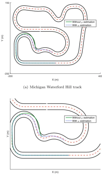
In the simulation, the vehicle is driven along a section of the Waterford Hill track, which contains a sharp bend. The adhesion coefficient (road surface) is set to the category

’dry’ from the beginning to the second bend. From the second bend the road surface is set to the category ’icy’. The simulation has been performed twice.

In the first case, the vehicle is driven by a nominal controller without information about the road surface. Whilst, in the second run, the car is controlled by the proposed control algorithm. The paths of the vehicle are illustrated in Figure 3. It can be seen that the vehicle, which is controlled by the nominal controller, leaves the road at the second bend, where the type of the road surface changes. However, the car, which is driven by the proposed algorithm, is able to follow the track despite the change in the road surface.

-200 400

X (m) -250

150

Y (m)

Without esitmation With estimation

(a) Michigan Waterford Hill track

X (m)

Y (m)

Without esitmation With estimation

(b) Section of the track

Fig. 3. Paths of the vehicle

The design of the LPV control requires the system dy- namics in the state-space form (8) and the performance equation (12). Moreover, it is necessary to scale the input and output signals of the plant, as it is illustrated in Figure 2. In practice, the scaling of the signals during the design process is performed through transfer functions G´asp´ar et al. [2017]. The role of Wref,1, Wref,2 is to scale the signals yref, ˙ψref. Similarly, Ww,1, Ww,2 scale the noises on the lateral position and on the yaw-rate measure- ments. Noises wy and wψ˙ are incorporated in the vector w=r wy wψ˙

^T

. The priority among the performances is guaranteed byWref,i,i={1,2,3}. The transfer functions Wref,i, i = {1,2} are selected in a second-order form to reach the smooth tracking of the reference signals. How- ever, in case of Wref,3 a first-order proportional transfer function can be enough to guarantee the minimization of δ.

P(ρ)

K(ρ)

data analysis

ρ surface estimation

Wref,1

Wref,2

yref

ψ˙ref

y ψ˙ δ

Wz,1

Wz,2

Wz,3

z1

z2

z3

Ww,1

Ww,2

wy

wψ˙

Fig. 2. Closed-loop interconnection structure

The quadratic LPV performance problem is to choose the parameter-varying controllerK(ρ) in such a way that the resulting closed-loop system is quadratically stable and the induced L² norm from the disturbance and the performances is less than the value γ. The minimization task is the following:

K(ρ)inf sup

ρ∈Fρ

sup

w2=0,w∈L2

z2

w2

, (13)

where Fρ bounds the scheduling variables. The yielded controllerK(ρ) is formed as

˙

xK=AK(ρ)xK+BK(ρ)yK, (14a) u=CK(ρ)xK+DK(ρ)yK, (14b) where xK is the state vector of the dynamic controller, AK, BK, CK, DK areρdependent matrices.

yK is the vector of the lateral error and yaw-rate error measurements, which is formed as

yK =C2x+D21r, (15) whereC2, D21are matrices.

The existence of a controller that solves the quadratic LPV γ-performance problem can be expressed as the feasibility of a set of LMIs, which can be solved numerically. The constraints set by the LMIs are not finite. The infiniteness of the constraints is relieved by a finite, sufficiently fine grid. To specify the grid of the performance weights for the LPV design the scheduling variables are defined through lookup-tables, see Wu et al. [1996], Szab´o et al. [2011].

5. SIMULATION EXAMPLE

In the last section, a comprehensive simulation example is presented to show the efficiency and the operation of the proposed control system.

In the simulation, the vehicle is driven along a section of the Waterford Hill track, which contains a sharp bend. The adhesion coefficient (road surface) is set to the category

’dry’ from the beginning to the second bend. From the second bend the road surface is set to the category ’icy’.

The simulation has been performed twice.

In the first case, the vehicle is driven by a nominal controller without information about the road surface.

Whilst, in the second run, the car is controlled by the proposed control algorithm. The paths of the vehicle are illustrated in Figure 3. It can be seen that the vehicle, which is controlled by the nominal controller, leaves the road at the second bend, where the type of the road surface changes. However, the car, which is driven by the proposed algorithm, is able to follow the track despite the change in the road surface.

-200 400

X (m) -250

150

Y (m)

Without esitmation With estimation

(a) Michigan Waterford Hill track

X (m)

Y (m)

Without esitmation With estimation

(b) Section of the track

Fig. 3. Paths of the vehicle

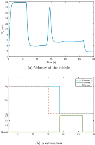
The velocity of the car varies during the simulations, as depicted in Figure 5(a). Furthermore, the result of the road surface estimation can be found in Figure 5 (b). As the figure shows, initially, the road surface is set to ’dry’ and it changes after 25s. The algorithm frequently yields ’No data’ category, which means that the µis not close to its peak value, therefore the estimation cannot be executed.

Figure 5 shows, when the vehicle reaches the lowµsegment

0 5 10 15 20 25 30

Time (s) 10

12 14 16 18 20 22 24 26 28 30

Vx (m/s)

(a) Velocity of the vehicle

5 10 15 20 25 30

No data 0.1 0.2 0.3Icy Wet Dry

Estimated Corrected Reference

(b)µestimation

Fig. 4. Velocity profile andµestimation

the value ofµis close to its peak value, and the estimation algorithm provides ’icy’, which is a correct classification.

At that moment, the control system reconfigures itself and adjust its parameters to the current road surface. It is the reason, why the vehicle does not leave the road at the second bend.

Finally in Figure 5, the calculated steering angle and the yaw-rate tracking are illustrated. As the figure indicates the tracking of the yaw-rate is accurate, the maximum of the tracking delay is below 0.3s.

6. CONCLUSIONS

In this paper, a new big-data based road surface estimation algorithm has been presented. The result of this algorithm has been built-in the lateral control design as a scheduling parameter. Moreover, a novel selection criterion has been presented, which was able to separate the instances, in which the adhesion coefficient was close to its peak value.

The comprehensive simulation study has been presented

0 5 10 15 20 25 30

Time (s) -2

-1.5 -1 -0.5 0 0.5 1 1.5 2 2.5

(deg)

(a) Steering angle

0 5 10 15 20 25 30

Time (s) -0.4

-0.3 -0.2 -0.1 0 0.1 0.2 0.3 0.4

Reference Vehicle

(b) Yaw-rate tracking

Fig. 5. Control actuation and yaw-rate tracking

that the proposed control system has a high effectiveness in the handling of the road surface variations.

REFERENCES

Daniel Fenyes, Balazs Nemeth, and Peter Gaspar. Analysis of autonomous vehicle dynamics based on the big data approach.European Control Conference, pages 219–224, 2018.

P´eter G´asp´ar, Zolt´an Szab´o, J´ozsef Bokor, and Bal´azs N´emeth.Robust Control Design for Active Driver Assis- tance Systems. A Linear-Parameter-Varying Approach.

Springer Verlag, 2017.

Md. Mushfiqul Islam, Muhammad Sheikh Sadi, Md. Milon Islam, and Md. Kamrul Hasan. A new method for road surface detection.2018 4th International Conference on Electrical Engineering and Information and Communi- cation Technology (iCEEiCT), 2018.

Shoutao Li, Xinglong Pei, and Yongxue Ma. A new road friction coefficient estimation method based on svm.

2012 IEEE International Conference on Mechatronics and Automation, pages 1910–1914, 2012.

Steffen M¨uller, Micheal Uchanski, and Karl Hedrick. Es- timation of the maximum tire-road friction coefficient.

Journal of dynamic systems, measurement and control, 125:607–617, 2003.

R. Rajamani. Vehicle dynamics and control. Springer, 2005.

J.J. Rath, K.C. Veluvolu, D. Zhang, Q. Zhang, and M. De- foort. Estimation of road adhesion using higher-order

sliding mode observer for torsional tyre model. 6th International Conference, pages 202–213, 2013.

Tao Song, Hongliang Zhou, and Haifeng Liu. Road friction estimation based on bp neural network. 36th Chinese Control Conference, pages 9491–9496, 2017.

Z. Sun and K. Jia. Road surface condition classification based on color and texture information.Annual Reviews in Control, 45:76–86, 2018.

Z. Szab´o, A. Marcos, D. P. Mostaza, M. Kerr, G. R¨od¨onyi, J. Bokor, and S. Bennani. Development of an inte- grated LPV/LFT framework: modeling and data-based validation tool. IEEE Transactions on Control Systems Technology, 19(1):104–117, 2011.

Yong Wang and Ian H. Witten.Pace Regression. (Working paper 99/12). Hamilton, New Zealand: University of Waikato, Department of Computer Science., 1999.

F. Wu, X.H. Yang, A. Packard, and G. Becker. Induced L2

norm controller forLPV systems with bounded param- eter variation rates. Journal of Robust and Nonlinear Control, 6:983–988, 1996.

sliding mode observer for torsional tyre model. 6th International Conference, pages 202–213, 2013.

Tao Song, Hongliang Zhou, and Haifeng Liu. Road friction estimation based on bp neural network. 36th Chinese Control Conference, pages 9491–9496, 2017.

Z. Sun and K. Jia. Road surface condition classification based on color and texture information.Annual Reviews in Control, 45:76–86, 2018.

Z. Szab´o, A. Marcos, D. P. Mostaza, M. Kerr, G. R¨od¨onyi, J. Bokor, and S. Bennani. Development of an inte- grated LPV/LFT framework: modeling and data-based validation tool. IEEE Transactions on Control Systems Technology, 19(1):104–117, 2011.

Yong Wang and Ian H. Witten.Pace Regression. (Working paper 99/12). Hamilton, New Zealand: University of Waikato, Department of Computer Science., 1999.

F. Wu, X.H. Yang, A. Packard, and G. Becker. Induced L2

norm controller forLPVsystems with bounded param- eter variation rates. Journal of Robust and Nonlinear Control, 6:983–988, 1996.