LPV based data-driven modeling and control design for autonomous vehicles
D´aniel F´enyes, Bal´azs N´emeth and P´eter G´asp´ar
Abstract— This paper provides a data-driven model-based solution for control problem of path following for autonomous vehicles. The modeling of the system is based on the Linear Parameter-Varying (LPV) framework, but the selections of the scheduling variables and the LPV model parameters are based on machine learning methods. The advantage of the method is that the performances of the system can be guaranteed, while the generated model is valid in an extended operation range.
The control design is based on the LPV method, in which the novel vehicle model is incorporated. The effectiveness of the method is illustrated through comparative simulation scenarios in CarMaker simulation environment.
I. INTRODUCTION AND MOTIVATION
A challenge in the era of the self-driving vehicles is that the vehicles must handle various situations autonomously.
At the top level of the automation the supervising role of humans is not requested, which significantly differs from the currently used driver assistance systems. The reliable solutions on several tasks must be incorporated in the control system, e.g. environment sensing, decision making or the changing of the vehicle dynamics due to the vehicle-road- environment interactions.
This paper focuses on the last task such as the adaption of the vehicle control to changeable vehicle dynamic scenarios.
An appropriate adaptation requires the intervention of the control system in wide range of the vehicle dynamics.
Nevertheless, the physical-based linear modeling and control solutions of the driver assistant systems can be insufficient for the autonomous actuation. Due to the linear approxima- tion several important safety features cannot be considered in the design. Moreover, the values of the physical parameters can vary during the lifetime of the vehicle.
A solution of the problem is to consider the nonlinearities in the vehicle dynamics through physical relationships, see e.g. [1], [2], [3]. A drawback of the solution is that it can be difficult to formulate and to involve the nonlinear characteristics in the control design. Another approach is to learn the dynamics of the vehicle through a machine
D. F´enyes, B. N´emeth, P. G´asp´ar are with Systems and Control Laboratory, Institute for Computer Science and Control, Kende u. 13-17, H-1111 Budapest, Hungary. E-mail:
[daniel.fenyes;balazs.nemeth;peter.gaspar]@sztaki.hu
This work has been supported by the research program titled ’Exploring the Mathematical Foundations of Artificial Intelligence’ under grant No.
2018-1.2.1-NKP-00008).
The work of Bal´azs N´emeth was partially supported by the J´anos Bolyai Research Scholarship of the Hungarian Academy of Sciences and the ´UNKP-19-4 New National Excellence Program of the Ministry for Innovation and Technology. The work of D´aniel F´enyes was partially supported by the ´UNKP-19-3 New National Excellence Program of the Ministry for Innovation and Technology.
learning algorithm, which produces e.g. a neural network based controller [4], [5] and decision logic [6]. Although machine learning methods can have promising results in the vehicle control, these solutions do not provide theoretical guarantees about the stability and performance issues of the closed-loop system.
This paper provides a data-driven model-based solution for the specific challenge of the vehicle path following. The structure of the controller is based on the general framework of the Linear Parameter-Varying (LPV) approach, but the selection of the scheduling variables and the LPV model parameters are based on machine learning methods. Using this mixed method the performances can be guaranteed, while the data-driven approach can provide the appropriate intervention of the control system in the extended range of vehicle dynamics.
There are some control design solutions, whose concepts are close to the proposed idea of this paper. For example, [7] presents a model predictive control solution, in which the terminal cost and the terminal set of the control problem are learned through iterations. In this idea the model of the system is based on physical principles with its limitations.
Model-free control methods are presented e.g. in [8], [9]. The advantage of these solutions is that preliminary information about the model structure for the control is not necessary.
Although in the variables of the model-free solutions several nonlinear features of the dynamics can be incorporated, they can provide conservative control interventions.
In the proposed novel solution the structure of the physical model is preserved, which makes the formulation of the performance requirements easier. For the selection of the scheduling variables a decision tree using a machine learning algorithm has been generated based on big data. Moreover, the computation of the model parameters is based on an optimization algorithm.
The contribution of the method is a big data-driven mod- eling process for LPV systems, whose result is applied in the robust control design. The proposed method is independent from the vehicle-oriented application and the properties of the dynamics. But, in this paper the approach is presented through the autonomous path following control of the lateral vehicle dynamics. The result of the method is a controller, which is able to handle the variation of the vehicle dynamic scenarios in a wide range. The effectiveness of the method in the extended range is illustrated through simulation in CarMaker environment.
2020 European Control Conference (ECC) May 12-15, 2020. Saint Petersburg, Russia
CarM aker
N ominal model
Scaling and categorization Machine
Learning LP V
controller
P reprocess of data Simulation
environment
States
Control signal
signalReference Measured
LP V Model identif ication
ofvehicle States
of model
Error
function
Schedulingpar.
Calculatedmodels variables
M odel identif ication Control design
Fig. 1. Methodological process for modeling, control design and evaluation
Structure of modeling and control process
In the rest of the section an overview about the modeling and control design process is provided. The method involves several subtasks, which are illustrated in Figure 1. The modeling and control subtasks can be divided into four main groups, such as: Prepocess of data, Model identification, Control design, data acquisition and implementation using theSimulation environment.
The layer ’Simulation environment’ contains the vehicle dynamic simulation software. It has role in the data acquisi- tion process for the machine learning algorithm, e.g. training and test sets. Moreover, it is used for the evaluation of the designed controller. In this paper the high-fidelity CarMaker software is used for this purpose.
The role of the layer ’Preprocess of data’ is to produce the training and test sets from the collected data. It scales the data and it also orders them into various categories. The results of the layer are training and test sets, which are ready for the supervised learning process. The methods behind the layer are presented in Subsections II-A and II-B.
The ’Model identification’ layer uses the provided labeled sets to determine the scheduling variables of the system. It requires the selection of the variables, which has significant impact on the dynamics of the vehicle. Moreover, in this layer the parameters of the LPV based vehicle model are calculated. The solution of the identification is found in Subsections II-C and II-D.
In the layer ’Control design’ the LPV controller based on the resulted model is designed. The performances of the controller is evaluated by using the ’Simulation environ- ment’. The results of the simulation scenarios are presented in Section IV.
II. DATA-DRIVEN MODELING PROCESS OF THELPV
SYSTEMS
This section focuses on the modeling process of the lateral vehicle dynamics in LPV form. The data collection, the method of the preprocessing, the selection of the schedul- ing variables through machine learning and the parameter identification problems are detailed below.
A. Acquisition of data from simulations
The layer ’Simulation environment’ must provide numer- ous simulations for the learning process. Since the learning requires variation in high range of the vehicle operation, several parameters of the vehicle and its environment have been modified in order to cover a wide range of the dynamics of the vehicle. For example, the longitudinal velocity varied between10−20m/sand the car were driven on tracks with different circuits. During the simulations all variables are measured, which are considered to be available from an on- broad system:
1) Longitudinal velocity (vx) 2) Angular velocity of the wheels
(ωx,y),x∈ {f ront, rear},y∈ {lef t, right}
3) Steering angle (δ) 4) Yaw-rate (ψ)˙
5) Accelerations (ax,ay)
6) Side-slip angle (β). Since the measurement of β can be difficult and expensive, this signal is only used for building up the model. During the operation of the control system it is not required.
The sampling time of the measurements has been set to Ts= 0.01sec. In this manner, more than10million distinct instances have been collected.
B. Labeling the elements of the collected dataset
The learning of the vehicle dynamics requires the scaling and the ordering of labels of the collected data. The goal of the labeling is to provide categories, with which the charac- teristics of the nonlinear vehicle motion can be distinguished from each other. These results yield training and test sets, which are ready for the supervised learning process.
The labeling of the vehicle dynamic signals is based on their deviation from the signals of a nominal, physical model, which is described by the physical model of the vehicle [10]:
Iψ¨=C1α1l1−C2α2l2 (1) mvx( ˙ψ+ ˙β) =C1α1+C2α2 (2) whereI denotes the yaw-inertia,C1, C2represent cornering stiffness, l1, l2 are the distances between the COG and the axles, α1, α2 are the side-slip angles of the front and rear wheels, which are calculated asα1=δ−β−ψlv˙1
x andα2=
−β + ψlv˙2
x. Moreover, ψ˙ is yaw rate, β is side-slip of the vehicle and vx is the longitudinal velocity of the vehicle, whileδ denotes steering angle.
The computation of the nominal, physical model signals require the state-space representation of the system x˙ = Apx+Bpu, whose state vector isx=ψ˙ βT
, the control input is the steering angleu=δandAp, Bpare matrices of the physical model. This representation is transformed to a discrete representation through the sampling timeTs= 0.01, which is the same as the sampling time of the measurements.
Using the measured input signalδ, the outputs of the discrete system are computed for each measurement point.
The labeling of the collected data is based on the deviation of the measured signals from the signals of the nominal
system. In this process the yaw-rate and the side-slip angles are involved, which are the independent states of the physical system. The labeling is based on the relative errors of the signals in timeti, such as
ψ˙e(ti) = |ψ˙m(ti)−ψ˙n(ti)|
ψ˙n(ti) (3a) βe(ti) = |βm(ti)−βn(ti)|
βn(ti) (3b) where ψ˙m and βm denote the measured outputs while ψ˙n
andβn are the outputs of the nominal system. In the method categories have been predefined for the classification of the instances, such asnequidistant sections between0and1. It is defined a functionf, which associates the errors (3) with the categories. A given instance inti is labeled based on the following value
cat(ti) = max
f ψ˙e(ti)
,f βe(ti)
, (4)
which means that the label cat(ti) is determined based on the maximum of the errors.
C. Selection of the scheduling variables
The selection of the scheduling variables of the LPV system is based on a decision tree algorithm. The role of the decision tree is to determine the most influential attributes using the previously labeled sets with cat. The main advantage of the decision trees is that they are able to provide reliable models even though the dataset has a highly nonlinear structure. In this paper the C4.5 decision tree algorithm is applied [11], [12]. The output of the decision tree is the category of a given instanceξ, which is used as scheduling parameter.
The method C4.5 requires two sets of data, which are generated from the datasetS: a training set and a test set. The training set is based on the collected data set, and it is used for building the decision tree, while the test set is used for the evaluation. The purpose of the C4.5 algorithm is to create a set of rules (decision tree), by which the instances can be correctly classified according to the selected dependent (class) attribute. The created set of rules is ordered into a tree structure. A decision tree consists of leaves, nodes and branches. A node is associated with a condition (e.g. current value of an attribute is smaller/bigger than a given value). A branch is the outcome of a node (the condition is satisfied or not) and leads to another node or to a leaf. Finally, a leaf determines the class of the instance.
In the given data-driven vehicle modeling problem, the leaves of the decision tree are associated with specific categories cat. The resulted tree classifies the instances by using only the measured actual attributes. The output of the decision tree isξ, which has the valuecatfor a specific leaf.
The parameter ξ is used as a scheduling variable of the system. The values of ξ, which represent categories, can be considered as a linear operating point of the nonlinear system. Figure 2 illustrates an example of the results. It can be seen that the location of the resulted categories
(represented by different colors) in the plot of the side-slip and the lateral force on the wheel are well distinguished. The shape of the function is close to the tire force characteristics, see [10]. It means that the machine learning algorithm is able to distinguish various sections, which are related to the levels of the relative errors (3).
Fig. 2. Illustration of the calculated categories
D. Parameter selection of the LPV model
The identification of the LPV system requires the selection of the parameters for each segments. For each segments a linear system can be adjusted and they create a gridded LPV system. The structure of the system is determined by the number of the states, which is derived from the physical model (1). In case of the lateral dynamics the data-driven system model is formed as
˙
xd =Ad(ξ)xd+Bdud(ξ), (5) where
Ad(ξ) =
a11(ξ) a12(ξ) a21(ξ) a22(ξ)
, Bd(ξ) = b1(ξ)
b2(ξ)
, and a11(ξ), a12(ξ), a21(ξ), a22(ξ) and b1(ξ), b2(ξ) are pa- rameters and the state-vector of the system is xd= [ ˙ψi βi], the control input isud=δ.
The lateral position of the vehicleyis computed by using the statesψ˙ andβ. The lateral acceleration v˙y is
˙
vy=vx( ˙ψ+ ˙β) =
=vxψ˙+vx(a21(ξ) ˙ψ+a22(ξ)β+b2(ξ)δ). (6) The identified system description is augmented as:
˙
x=A(ρ)x+B(ρ)u (7) and
A(ρ) =
a11(ξ) a12(ξ) 0 0 a21(ξ) a22(ξ) 0 0 vx(1 +a21(ξ)) vxa22(ξ) 0 0
0 0 1 0
, B(ρ) =
b1(ξ) b2(ξ) vxb2(ξ)
0
,
where the state vector of the system is x = ψ˙ β vy yT
, the input isu=ud, moreover, the vector of the scheduling variables isρ=
ξ vx .
The purpose of the identification is to find the parameters a11(ξ), a12(ξ), a21(ξ), a22(ξ) and b1(ξ), b2(ξ), with which
the results of the state calculationxare close to the measured states xm. It leads to an optimization problem, which is formed as:
a11(ξ),a12(ξ),a21min(ξ),a22(ξ),b1(ξ),b2(ξ) xm(ti)−x(ti)2
(8) for all xm(ti) instances in all ti time step in the training set. During the solution of (8) the systems can be computed independently for fixed ξ values in the grids. Thus, the parameter-dependent quadratic optimization problem leads to a least-squares problem [13], [14]. The result of the optimization is a set of polytopic systems, which represents the LPV description of the vehicle model.
III. PATH FOLLOWINGLPVCONTROL DESIGN USING THE DATA-DRIVEN MODEL
In this section a path following control design method is presented by using the identified data-driven vehicle model.
The control system is responsible for guaranteeing the trajec- tory tracking of the vehicle and minimizing the interventions.
The purpose of the control design are described by the following performances.
• Minimization of the lateral error: In order to reach good path following property, the control system has to minimize the lateral error between the roadyref and the lateral position of the vehicley:
z1=yref −y, |z1| →min, (9) where yref is determined by the selected route of the vehicle.
• Minimization of the yaw-rate error: Beside the lateral error, the controller has to reduce the error between the reference ψ˙ref and the measured yaw-rate ψ˙ in order to reach accurate and smooth tracking:
z2= ˙ψref −ψ,˙ |z2| →min, (10) whereψ˙ref is determined by the curvature of the route and the velocity of the vehicle, see [10].
• Minimization of the steering angle: The control system has to minimize its interventions to reduce the energy consumption:
z3=δ, |z3| →min. (11) The performances are summarized in the following vector z =
z1 z2 z3T
, which can be expressed in a perfor- mance equation
z=C1x+D11r+D12u, (12) where C1, D11, D12 are matrices and r contains the signal yref.
The model used for the control design is based on the data-driven model (7), the performance equation (12) and the measurement equation:
˙
x=Ax+Bu, (13a)
z=C1x+D11r+D12u, (13b)
yK =C2x, (13c)
where (13c) represents the measurement ofyK= y ψ˙
. In the LPV control design, the extended state-space model (13) is employed. Moreover, during the control design several weighting functions are used to scale the measured signals and to reach the specified performance level. The augmented plant with the weighting functions are illustrated in Figure 3.
The roles of the weighting functionsWref,1 andWref,2 are to scale the reference signalsyref andψ˙ref. FunctionsWz,1
andWz,2guarantee the accurate tracking performance of the vehicle, whileWz,3 scales the control intervention. Finally, the roles of the weighting functions Ww,1,Ww,2 andWw,3
are to scale the noises of the measured signals.
P(ρ)
K(ρ)
Decision Tree
Wref,2
ψ˙ref
y
δ
Wz,2
z2
Ww,1
Ww,3
wψ˙
wy˙
˙ y
Wz,3
z3
Ww,2
wy
ξ
Wz,1
z1
Wref,1
yref
ψ˙
Model
Measuredattributes
vx
Fig. 3. Structure of LPV controller
The quadratic LPV performance problem is to choose the parameter-varying controller K(ρ) in such a way that the resulting closed-loop system is quadratically stable and the induced L2 norm from disturbance and to performances is less than the valueγ. The minimization task is the following:
inf
K(ρ) sup
ρ∈Fρ
sup
kwk26=0,w∈L2
kzk2
kwk2, (14)
where Fρ bounds the scheduling variables. The yielded controllerK(ρ)is formed as
˙
xK =AK(ρ)xK+BK(ρ)yK, (15a) u=CK(ρ)xK+DK(ρ)yK, (15b) where AK(ρ), BK(ρ), CK(ρ), DK(ρ) are variable- dependent matrices.
IV. SIMULATION RESULTS
In this section a simulation example is presented to show the operation and the effectiveness of the proposed control system. The example presents the results of the decision tree generation, the selection of the weighting functions in the control design and the evaluation of the designed controller through a comparative vehicle dynamic scenario.
In the generation of the decision tree the number of the categories of the error is set to n = 6, which means that the values of the error function are divided into 6 groups.
Using these groups, several decisions have been created and their results are summarized in Table I. The first column of Table I shows the signals, which are used by the given decision tree. The second column represents the number of
the minimal objects, which influences the size of the tree.
Third column gives the percentage of the correctly classified instances. As a contribution, the best result is produced by the largest tree, which consists of almost 70 elements. However, due to the increased size it is not recommended to use in practice. Therefore in the fourth case, the tree uses only two signals (δ,ψ) and it also leads to an appropriate classification˙ capability with more than 94%. In the rest of the example the setting of the fourth tree is selected.
TABLE I
RELATIONSHIP BETWEEN THE TREE SIZE AND ITS CORRECTNESS Signals Min. obj. Corr. Class. Inst. Size δ,ψ, a˙ x, ωf l, ωrr 500 98.1% 69 δ,ψ, a˙ x, ωf l, ωrr 1000 97.5% 41 δ,ψ, a˙ x, ωf l, ωrr 2000 96.7% 33
δ,ψ˙ 5000 94.5% 17
δ,ψ˙ 10000 93.7% 11
Table II illustrates the corresponding confusion matrix, which represents the percentages of the classification for all scenarios. The first row represents the output of the decision tree, while the last column shows the correct class of the instances. It is shown that the misclassification is rare.
Moreover, the misclassified instances are usually only 1 class away from the correct class. The designed decision tree has a appropriate classification performance and it can be used effectively in selection of the scheduling variables.
TABLE II CONFUSION MATRIX
ξ= 1 ξ= 2 ξ= 3 ξ= 4 ξ= 5 ξ= 6
47.4 0.67 0 0 0 0 cat= 1
2 30.3 1.1 0 0 0 cat= 2
0 0.38 18.2 0.1 0 0 cat= 3
0 0 0.24 1.8 0 0 cat= 4
0 0 0 0.24 0.7 0 cat= 5
0 0 0.23 0 0 0.7 cat= 6
The design of the LPV controller requires the selection of the weighting functions, in which the disturbances and the reference signals are scaled and the performances are specified. In the given lateral vehicle control problem the weighting functions on the reference signals are selected as
Wref,1= 0.1
100s+ 1, Wref,2= 0.01
100s+ 1. (16) Furthermore, the role of functions Wz,1 and Wz,2 are to guarantee the accurate trajectory tracking of the vehicle:
Wz,1= 10 1−10n
s2+ 2s+ 1, Wz,2= 1
s+ 1. (17) Weighting functionWz,3scales the control intervention and it provides a balance between minimization in the control energy:
Wz,3= 0.011s+ 1
2s+ 1. (18)
The further three functions scales the noises on the measured signals, such as Ww,1 = 0.002, Ww,2 = 0.001, Ww,3 = 0.05.
In the following, a comparative simulation example is presented, in which the vehicle with different controllers and varying velocity is driven along a sharp bend with asphalt pavement. Firstly, the vehicle is controlled by a nominal LPV controller, which is designed based on the physical model of the vehicle withoutξ. In the second case the vehicle is driven by the proposed control system. Figure 4 shows the path of the vehicle in both cases and Figure 5 presents the variation of the velocity. It can be seen in Figure 4, when the vehicle is controlled by the nominal controller, it leaves the track at the beginning of the bend. However, when the car is driven by the proposed control algorithm, the vehicle is able to follow the track with a low lateral error.
-550 -500 -450 -400 -350 -300
X (m) 350
400 450 500 550 600 650 700
Y (m)
Track LPV controller Nominal controller
Fig. 4. Positions of the vehicles during the simulations
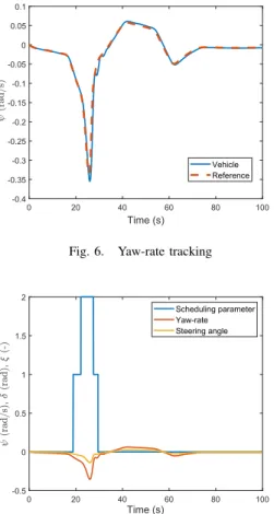
The performance of the yaw-rate tracking is illustrated in Figure 6. As it shows, the proposed control system can guarantee the yaw-rate tracking for varying velocities. The delay of the tracking is below a low value0.2sec.
The scheduling parameter ξ is calculated by using the selected decision tree. Based on the analysis in Table I, the chosen decision tree uses two signals: the steering angle and the yaw rate. Figure 7 illustrates the variation of ξ together withψ˙ andδ. The scheduling parameter covers three categories [0; 1; 2], which are associated with the specific
0 20 40 60 80 100
Time (s) 10
12 14 16 18 20 22 24 26 28
Vx (m/s)
Fig. 5. Velocity profile of the vehicles
0 20 40 60 80 100 Time (s)
-0.4 -0.35 -0.3 -0.25 -0.2 -0.15 -0.1 -0.05 0 0.05 0.1
Vehicle Reference
Fig. 6. Yaw-rate tracking
0 20 40 60 80 100
Time (s) -0.5
0 0.5 1 1.5 2
Scheduling parameter Yaw-rate Steering angle
Fig. 7. Scheduling variableξ
identified models. The decision tree yields the category 2 when the steering angle and the yaw-rate signals reach their peak values. By selecting the appropriate category, the stable motion and tracking performance of the vehicle can be guaranteed.
Finally, the resulting steering angle is illustrated separately in the Figure 8. As it shows, the values of the steering angle is between(−9,2deg), which is a physically reasonable range for the steering signal.
V. CONCLUSIONS
The simulation results has illustrated the operation of the proposed LPV control. The advantage of this solution is that the performances of the system can be guaranteed, while the generated model is valid in an extended operation range.
Through the collected big data scheduling variables of the system are selected, which represent the current nonlinear characteristics of the vehicle dynamics. The comparative example presented that the proposed data-driven modeling and control design method can be an alternative solution of the physical-based approaches.
REFERENCES
[1] G. Palmieri, M. Bari´c, L. Glielmo, and F. Borrelli, “Robust vehicle lateral stabilisation via set-based methods for uncertain piecewise affine systems,”Vehicle System Dynamics, vol. 50, no. 6, pp. 861–
882, 2012.
0 20 40 60 80 100
Time (s) -10
-8 -6 -4 -2 0 2
(deg)
Fig. 8. Steering angle
[2] B. N´emeth, P. G´asp´ar, and T. P´eni, “Nonlinear analysis of vehicle control actuations based on controlled invariant sets,”Int. J. Applied Mathematics and Computer Science, vol. 26, no. 1, 2016.
[3] M. I. Masouleh and D. J. N. Limebeer, “Non-linear vehicle domain of attraction analysis using sum-of-squares programming,” in2016 IEEE Conference on Control Applications (CCA), Sept 2016, pp. 1209–
1214.
[4] C. Hubschneider, A. Bauer, J. Doll, M. Weber, S. Klemm, F. Kuhnt, and J. M. Z¨ollner, “Integrating end-to-end learned steering into probabilistic autonomous driving,” in2017 IEEE 20th International Conference on Intelligent Transportation Systems (ITSC), Oct 2017, pp. 1–7.
[5] V. Rausch, A. Hansen, E. Solowjow, C. Liu, E. Kreuzer, and J. K.
Hedrick, “Learning a deep neural net policy for end-to-end control of autonomous vehicles,” in2017 American Control Conference (ACC), May 2017, pp. 4914–4919.
[6] L. Li, K. Ota, and M. Dong, “Humanlike driving: Empirical decision- making system for autonomous vehicles,” IEEE Transactions on Vehicular Technology, vol. 67, no. 8, pp. 6814–6823, Aug 2018.
[7] U. Rosolia and F. Borrelli, “Learning model predictive control for iterative tasks. a data-driven control framework,”IEEE Transactions on Automatic Control, vol. 63, no. 7, pp. 1883–1896, July 2018.
[8] M. Fliess and C. Join, “Model-free control,”International Journal of Control, vol. 86, no. 12, pp. 2228–2252, 2013.
[9] S. Formentin, P. De Filippi, M. Corno, M. Tanelli, and S. M. Savaresi,
“Data-driven design of braking control systems,”IEEE Transactions on Control Systems Technology, vol. 21, no. 1, pp. 186–193, Jan 2013.
[10] R. Rajamani, “Vehicle dynamics and control,”Springer, 2005.
[11] E. B. Hunt,Concept Learning: An information Processing Problem.
Wiley, 1962.
[12] J. R. Quinlan,C4.5: Programs for Machine Learning. San Mateo, California: Morgan Kaufmann Publishers, 1993.
[13] P. E. Gill, W. Murray, and M. Wright,Practical Optimization. Aca- demic Press, London UK, 1981.
[14] T. F. Coleman and Y. Li, “A reflective newton method for minimizing a quadratic function subject to bounds on some of the variables,”SIAM Journal on Optimization, vol. 6, no. 4, pp. 1040–1058, 1996.