A TP-LPV-LMI Approach to Control of Tumor Growth

(1)

of Tumor Growth

György Eigner and Levente Kovács

Abstract By using advanced control techniques to control physiological systems sophisticated control regimes can be realized. There are several challenges need to be solved in these approaches, however. Most of the time, the lack of information of the internal dynamics, the nonlinear behavior of the system to be controlled and the variabilities coming from that simple fact that people are different and their specifics vary in time makes the control design difficult. Nevertheless, the use of appropriate methodologies can facilitate to find solutions to them. In this study, our aim is to introduce different techniques and by combining them we show an effective way for control design with respect to physiological systems. Our solution stands on four pillars: transformation of the formulated model into control oriented model (COM) form; use the COM for linear parameter varying (LPV) kind modeling to handle unfavorable dynamics as linear dependencies; tensor product modeling (TPM) to downsize the computational costs both from modeling and control design viewpoint;

and finally, using linear matrix inequalities (LMI) based controller design to satisfy predefined requirements. The occurring TP-LPV-LMI controller is able to enforce a given, nonlinear system to behave as a selected reference system. In this study, the detailed control solution is applied for tumor growth control to maintain the volume of the tumor.

Keywords Tumor growth control

·

Linear parameter varying

·

Tensor product model transformation

This project has received funding from the European Research Council (ERC) under the European Union’s Horizon 2020 research and innovation programme (grant agreement No 679681).

G. Eigner·L. Kovács (

B

⁾

Physiological Controls Research Center, Research, Innovation and Service Center of Óbuda University, Budapest, Hungary

e-mail:kovacs@uni-obuda.hu G. Eigner

e-mail:eigner.gyorgy@nik.uni-obuda.hu

L. Kovács et al. (eds.),Recent Advances in Intelligent Engineering, Topics in Intelligent Engineering and Informatics 14,

https://doi.org/10.1007/978-3-030-14350-3_12

223

(2)

1 Introduction

The so-called Targeted Molecular Therapies (TMTs) are specific therapeutic oppor- tunities came into focus recently concerning the treatment of cancer. They have been successfully applied as therapeutic agents in treatment of different types of tumor moreover they are under investigation as complementary therapies as well regarding classical treatments such as surgery, chemotherapy, radiotherapy and so on. In general they affect the tumors by inhibiting specific biochemical which are respon- sible for the growth, spread and/or proliferation of tumor concourses [1,2]. Due to they block or inhibit the properties of tumors in a specific way more personalized therapies can be achieved [3]. Another aspect why TMTs could be good alterna- tive or complementary to conservative therapies is that they are less harmful them, causing less side effects while the load of the body becomes lower. Further they are able to increase the efficiency of regular therapies as well [1]. In the recent times many biochemical pathways have been discovered serving as a basis for TMT developments. The most commonly applied are the apoptosis inducers (facilitating the self-destruction of tumor cells), gene expression inhibitors (decreasing the protein expression in tumor cells which can be useful for the goals of tumor cells), signal transmission inhibitors (inhibiting the biochemical signaling capabilities of tumors) and anti-angiogenic therapies [3].

In this study we consider angiogen inhibition as the basis of therapy. Angiogen inhibitors affect the vascular endothelial growth factor (VEGF) which facilitates the proliferation concerning to the formation of new blood vessels. The process is es- sential for cancer concourses in order to get enough nutrients needed for further growing after the size of them reach a given volume (diffusion barrier) [4]. The tumors produce VEGF to facilitate the formation of new blood vessels through which the tumor populations can be supported with oxygen and nutrients. The inhibition of this pathway leads to insufficient nutrition from the tumor point of view and after time causing the “starvation” of the tumor [3,5]. The way of how this therapy works makes it an excellent therapeutic target and by combining with control engineering methodologies more optimized drug administration can be realized for a better treatment outcome [6]. Bevacizumab is one of the applied anti-angiogen TMT kind drugs considered in this study as well [4].

From the applicable control methods viewpoint several issues need to be over- bridged during the design. Alike well-known physiological control problems such as anesthesia or diabetes [7–11], the control of tumor growth is challenging. Several unfavorable effects need to be considered for example the nonlinear behavior of the phenomena to be controlled, the cross-effects, model and parameter uncertainties or even time-delay. Although, it is possible to find solutions suitable with respect to given requirements [6,12–16].

In this study we investigate a complex controller design approach that involves techniques from the latest developments of control engineering. We alloy the Lin- ear Parameter Variability (LPV) modeling technique with Linear Matrix Inequality (LMI) based controller design both formulated accordingly by Tensor Product (TP)

(3)

model transformation. The LPV framework is a useful technique by which model and parameter uncertainties can be handled moreover it allows the use of linear control design techniques without exact linearization [17–19]. In the recent decades the LMI based control design regarding the LPV framework became well-established especially with respect to state- and output-feedback kind controls. Most of the LMI theorems are based on the laws of Lyapunov [17, 20, 21]. The TP framework is extremely useful because of its ability to make the previously mentioned methods less conservative and the specific properties of the TP form representation makes the LMI based design easier [22–24]. The study investigates a specific TP-LPV-LMI kind controller class regarding tumor growth control. These controllers have many favorable properties for example the uncertainties and nonlinearities can be encap- sulated into the model structure leading an “intuitive” robust behavior of the control structure against sort of issues. Moreover the qualitative and quantitative control requirements can be formulated as LMIs through which the designed controller is able to satisfy them [17,20].

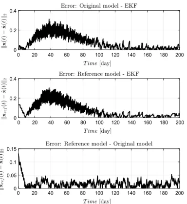
During our research state-feedback kind control has applied which requires internal information regarding the state variables during operation. In order to deal with the problem we applied an LPV based Extended Kalman Filter (EKF) solution as an estimator of the state variables. The designed EKF is able to provide the necessary information even though the circumstances [25].

This study is structured in the following way. First we introduce the modeling parts of the research concern to the applied nonlinear tumor growth model, reference model and developed qLPV models. After the controller design is presented including the TP model transformation and the applied LMIs. Then our results are showed and discussed. Finally, we conclude our research and formulate some hints regarding our future work.

2 Modeling Assumptions

2.1 Investigated Tumor Growth Model

We have applied the modified version of the extended Hahnfeldt-model in this study in accordance with the research goals [6, 16, 26]. The extended model takes into account the absorption dynamics of the inhibitor as well as it is described by (3).

The model has three ordinary differential equations [6]:

˙

z₁(t)= −λ1z₁(t)ln z₁(t)

z2(t)

, (1)

˙

z₂(t)=bz₁(t)−d z^2/3₁ (t)z2(t)−ηz2(t)z3(t) , (2)

˙

z3(t)= −λ3z3(t)+u(t) . (3)

(4)

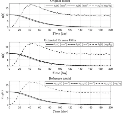
The model consists of three state variables: the tumor volumez1(t)[mm³], the sup- porting vasculature volumez2(t)[mm³] and the inhibitor serum levelz3(t)[mg/kg], respectively. The considered measurable output is the tumor volumez1(t)[mm³].

The following parameter set has been applied during our investigations:λ1=0.1921 1/day,b=5.851 1/day,d =0.00871 1/(mm²day),η=0.66 kg/(mg day) based on [26]. Theλ3=1.31 1/day clearance rate belongs to the assumed inhibitor (endo- statin) [26].

One has to emphasize that the model has a crucial limitation regarding numerical stability and the border of feasibility. Whenz₁andz₂state variables are approaching zero the ln

z₁(t) z2(t)

part of (1) tend to 0/0 kind singularity that should be avoided during operation.

As it was proven in [14, 16] by transforming the model the aforementioned issue can be converted into a more suitable form. The z_1,2(t)state variables can be transformed and new state variables can be introduced as x₁(t)=ln(z₁(t)), x₂(t)=ln(z₂(t)). The third state variable is linear and not necessary to be transformed so that isx₃(t)=z₃(t). The new model equations of the extended transformed model of Hahnfeldt can be written in the following way [16]:

˙

x1(t)= −λ1x1(t)+λ1x2(t) , (4)

˙

x₂(t)=be^x¹⁽^t⁾⁻^x²⁽^t⁾−de^2x¹⁽^t^)/3−ηx₃(t) , (5)

˙

x3(t)= −λ3x3(t)+u(t) . (6) In order to map the operating domain of the state variables we have to examine (1)–

(3) as first step. There is a limitation regardingz1andz2. The nontrivial equilibrium of the model can be calculated by rearranging (1)–(3) equations. The assumption of permanent inhibitor levelz₃(t)≡z_3,∞leads to the following results [6,27]:

z_1,∞=z_2,∞=

b−ηz3,∞

d

_3/2 , z_1,max=z_2,max =

b d

_3/2

↔z_3,∞= 1 λ3

u_∞≡0.

(7)

Equation (7) shows that the operating domain of z1 andz2 original state variables are z1(t),z2∈

0, (b/d)^3/2

[mm³]. In this study we assumed z1(t),z2∈ 1, (b/d)^3/2

[mm³]. This corresponds to the physiological fact that by using only the anti-angiogenic therapy the tumor cannot be totally eliminated moreover this is in conjunction with our previous findings [6]. The numerical instability can also be avoided in this way. Therefore the operating domain of the transformed state variables becomesx1,x2∈

ln(1),ln((b/d)³^/²)

=

0,9.7648 .

Accordingly, the goal of the control can be predefined as x₁=x₂ →0 when t →tendwhich is equivalent toz₁=z₂→1 whent→tend. With other words, the

(5)

“numerical goals” of the control related to the final values of the states arex_1,2,∞≡0 andz_1,2,∞≡1.

It should be noted that the extended transformed model is applied for the controller design—moreover, the EKF is also based on the extended transformed model.

2.2 Control Oriented Model Form

A given state space model can be written in control oriented model form [17,28].

That means the state variables of the model are transformed by using a shift operation. The transformed model describes the deviation between a given model equi- libriumxequili br i um or reference trajectoryxr e f(t)and the actual state variablesx(t).

Namely, it models the so-called “error dynamics”. By assuming that the shifted difference based state variables describe the deviation between xr e f(t) and x(t) the transformation is the following:Δx(t)=x(t)−xr e f(t). Naturally, the output, input, disturbances and noises should be transformed if they are interpreted during the controller design, namely,Δy(t)=y(t)−yr e f(t),Δu(t)=u(t)−ur e f(t), Δd(t)=d(t)−dr e f(t),Δn(t)=n(t)−nr e f(t).

In case of state-feedback kind controller, the control goal is to enforce the state variables to reach zero. This cannot be directly used in this case. However, by applying the control oriented model form in case of state-feedback the control goal is to enforce the shifted difference based state variables to reach zero—which is equivalent that the state variables of the reference model and the model to be controlled are equal.

With other words to eliminate theΔx(t)over time asΔx(t)→0,t →tend. This is equivalent with enforcing the model to behave as the selected reference model (Δx(t)=0≡x(t)=xr e f(t)).

2.3 Development of the Reference Model

Due to onlyx1(t)is considered as measurable the reference model has to be based on this state variable. In addition thex_1,r e f(t)has to be as simple as possible and it should describe a smoothly decreasing state trajectory. For that reason, we have developed the following reference model:

x1,r e f(t)=e^(−ξ·^t⁾·x1,r e f(t0) , (8)

where the numerical value of ξ scalar determines the velocity of decay and t is the time. The initial value xr e f(t0)is assumed to be known. The initial value can be derived by using measurements (then x1(t0)=x1,r e f(t0)) or estimations (then

ˆ

x1(t0)=x1,r e f(t0)). The reference model will serve as a basis for trajectory planning as it is detailed at the controller design.

In this studyξ =0.05 was applied.

(6)

3 LPV Modeling

A general parameter varying dynamical system can be described as follows [29]:

S=(T,P,W,B) , (9) where S is the LPV system,Tis the time series,Pis the scheduling space,Wis the signal space andB∈(W×P)^Tis the behavior of the system ((W×P)^Tis the collection of all possible maps fromTtoW×P).

In conformity with [30–32], the general state-space form of an LPV model is the following:

˙

x(t)=A(p(t))x(t)+B(p(t))u(t) y(t)=C(p(t))x(t)+D(p(t))u(t) S≡S(p(t))=

A(p(t))B(p(t)) C(p(t))D(p(t)) x(t)˙

y(t)

=S(p(t)) x(t)

u(t)

. (10)

The considered vectors and parameter dependent matrices are:x(t)∈Rⁿstate vector, u(t)∈R^m input vector, y(t)∈R^k output vector, A(p(t))∈Rⁿ^×ⁿ state matrix,B(p(t))∈Rⁿ^×^minput matrix,C(p(t))∈R^k^×ⁿoutput matrix,D(p(t))∈R^k^×^m feed-forward matrix andS(p(t))∈R⁽ⁿ⁺^k^)×(ⁿ⁺^m⁾system matrix. The matrices in (5) are dependent from the p(t)∈Ω^R ∈R^R parameter vector which consists of the so-called scheduling variables pi(t), namely,p(t)= [p₁(t) . . .pR(t)]. TheΩ = [p_1,mi n,p_1,max] × [p_2,mi n,p_2,max] × · · · × [pR,mi n,pR,max] ∈R^R hypercube—a subspace of theR^Rreal vector space—is characterized by the extremes of thepi(t). An LPV model inasmuch any of the state variables are involved into the scheduling parameters it is called qLPV model [31].

3.1 qLPV Model Development

During the qLPV modeling we use the assumptions of Sect.2.2. The transformation of the first and third state variables are equivocal—since the (4) and (6) are linear equations.

The transformations can be done as follows:

Δx˙1(t)= ˙x1(t)− ˙x_1,r e f(t)= −λ1x1(t)+λ1x2(t)−

−λ1x_1,r e f(t)+λ1x_2,r e f(t) =

−λ1(x1(t)−x_1,r e f(t))+λ1(x2(t)−x_2,r e f(t))=

−λ1Δx1(t)+λ1Δx2(t).

(11)

(7)

Δx˙₃(t)= ˙x₃(t)− ˙x_3,r e f(t)=

−λ3x₃(t)+u(t)−

−λ3x_3,r e f(t)+ur e f(t) =

−λ3Δx₃(t)+Δu(t).

(12)

Due to the exponential functions transformation of (5) it results:

Δx˙2(t)= ˙x2(t)− ˙x_2,r e f(t)= be^x¹⁽^t⁾⁻^x²⁽^t⁾−de^2x¹⁽^t^)/³−ηx3(t)

−

be^x^{1,r e f}⁽^t⁾⁻^x^{2,r e f}⁽^t⁾−de^2x^{1,r e f}⁽^t^)/³−ηx3,r e f(t). (13) In order to reach the desired qLPV form the following mathematical manipulations can be applied:

be^x¹⁽^t⁾e⁻^x²⁽^t⁾−be^x^{1,r e f}⁽^t⁾e⁻^x^{2,r e f}⁽^t⁾−0=

be^x¹⁽^t⁾e⁻^x²⁽^t⁾−be^x^{1,r e f}⁽^t⁾e⁻^x^{2,r e f}⁽^t⁾−be^x^{1,r e f}⁽^t⁾e⁻^x²⁽^t⁾ +be^x^{1,r e f}⁽^t⁾e⁻^x²⁽^t⁾=

be⁻^x²⁽^t⁾(e^x¹⁽^t⁾−e^x^{1,r e f}⁽^t⁾)·1

−be^x^{1,r e f}⁽^t⁾(e⁻^x²⁽^t⁾−e⁻^x^{2,r e f}⁽^t⁾)·1= be⁻^x²⁽^t⁾(e^x¹⁽^t⁾−e^x^{1,r e f}⁽^t⁾)

Δx1(t) Δx1(t)

−be^x^{1,r e f}⁽^t⁾(e⁻^x²⁽^t⁾−e⁻^x^{2,r e f}⁽^t⁾) Δx2(t) Δx₂(t)

−de^2x¹⁽^t^)/3+de^2x¹^,^{r e f}⁽^t^)/3=

−d

e^2x¹⁽^t^)/3−e^2x^{1,r e f}⁽^t^)/3 ·1=

−d

e^2x¹⁽^t^)/3−e^2x^{1,r e f}⁽^t^)/3

Δx₁(t) Δx1(t).

−ηx₃(t)+ηx_3,r e f(t)= −ηΔx₃(t).

(14)

From (12) two scheduling variables can be selected based on (14):

◦ p₁(t)=be⁻^x²⁽^t⁾

e^x^1(t)−e^x^{1,r e f}^(t) Δx₁(t) −d

e^2x^1(t)/3−e^2x^{1,r e f}^(t)/3 Δx₁(t)

◦ p2(t)= −be^x^{1,r e f}⁽^t^{) (}^e^−x^2(t)_Δ⁻_x^e₂⁻₍_t^x^{2,r e f}₎ ⁽^t⁾⁾

Accordingly, the transformedΔx2(t)state variable becomes:

Δx˙₂(t)= p₁(t)Δx₁(t)+p₂(t)Δx₂(t)−ηΔx₃(t) . (15) The p_1,2(t)has to be investigated from stability point of view since the divisions byΔx_1,2(t)in both terms may cause numerical instability whenΔx_1,2(t)→0. In order to decide what happens when Δx_1,2(t)→0 the L’Hospital’s rule [33] can be applied, namely, to calculate the finite final values (if any) of p₁(t)|_Δx1(t)=0and

p₂(t)|_Δx2(t)=0.

(8)

Δxlim₁(t)→0p1(t)= lim

Δx₁(t)→0 b e⁻^x²⁽^t⁾

e^x¹⁽^t⁾−e^x^{1,r e f}⁽^t⁾ Δx1(t)

−d

e^2x¹⁽^t^)/3−e^2x^{1,r e f}⁽^t^)/3

Δx1(t) =

e^x¹⁽^t⁾+e^x^{1,r e f}⁽^t⁾ 2

3d+be^2x²⁽^t⁾

.

Δxlim2(t)→0p2(t)= lim

Δx2(t)→0 be⁻^x^{1,r e f}⁽^t⁾(e^x²⁽^t⁾−e^x²^,^{r e f}⁽^t⁾) Δx2(t) =

−be^x^{1,r e f}⁽^t⁾

e^x²⁽^t⁾+e^x^{2,r e f}⁽^t⁾ .

(16)

By considering (15) these conditions has to be embedded into the implementation in the following way.

p₁(t)=

⎧⎪

⎪⎪

⎪⎨

⎪⎪

⎩ b e⁻^x²⁽^t⁾

e^x¹⁽^t⁾−e^x^{1,r e f}⁽^t⁾ Δx1(t)

−d

e^2x¹⁽^t^)/3−e^2x^{1,r e f}⁽^t^)/3

Δx1(t) , ifΔx1(t) =0 e^x¹⁽^t⁾+e^x^{1,r e f}⁽^t⁾ 2

3d+be^2x²⁽^t⁾

, ifΔx1(t)=0

(17)

p2(t)=

⎧⎨

⎩

be⁻^x^{1,r e f}⁽^t⁾(e^x²⁽^t⁾−e^x²^,^{r e f}⁽^t⁾)

Δx2(t) , ifΔx2(t) =0

−be^x^{1,r e f}⁽^t⁾

e^x²⁽^t⁾+e^x^{2,r e f}⁽^t⁾ , ifΔx2(t)=0

(18)

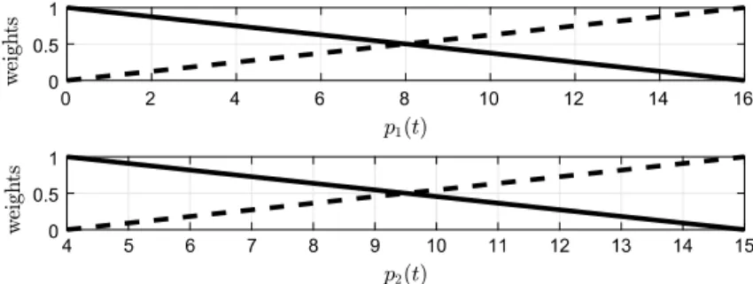
The operating domain of p(t) can be calculated based on (17)–(18) by considering the values of x1,2(t) and x1,2,r e f(t) which may appear during operation. Based on our experiments in the topic we found that the application of Ω = [p_1,mi n,p_1,max] × [p_2,mi n,p_2,max] = [0,16] × [4,15]domain can be applied, namely p1(t)= [0, . . . ,16]and p2(t)= [4, . . . ,15]. The reason is to take into account the physiological reasonable minimum and maximum numerical values of functions in (17)–(18).

The LPV model can be written in control oriented model form as with respect to Sect.2.2by considering (11), (12) and (15):

Δ˙x(t)=A(p(t))Δx(t)+BΔu(t) Δy(t)=CΔx(t)

S(p(t))=

A(p(t))B C 0

=

⎡

⎢⎢

⎣

−λ1 λ1 0 0 p1(t) p2(t) −η 0

0 0 −λ3 1

1 0 0 0

⎤

⎥⎥

⎦.

(19)

(9)

4 Control Design

4.1 TP Modeling and Control

The TP model transformation is a mathematical tool which is able to convert arbitrary—but appropriately formalized—qLPV model into TP model form. The resulting TP model approximates the qLPV model via the original nonlinear model as well with given accuracy depends on the sampling density applied onΩ. The TP model transformation has been successfully applied in several cases regarding nonlinear control problems (e.g. [23,28,34–36]). The TP model transformation can be directly applied on (10) and (19) [17]. The resulting finite element convex polytopic TP model is the following:

x(t˙ ) y(t)

=S(p(t)) x(t)

u(t)

S(p(t))=S ^R

r=1wr(pr(t))=S×rw(p(t))

, (20)

whereScore tensor composed ofS_i₁_,_i₂_,...,_i_RLTI vertices as_S∈R^I¹^×I²^×···×I^R×(n+k)×(n+m). Each of theSi1,i2,...,iR terms represents a given LTI system with different parameter set. The wr(pr(t)) weighting vector determines which LTI system dominates in the resulting S(p(t)). Thewr(pr(t))weighting vector function is composed of wr,ir(pr(t)) (ir =1. . .IR)continuous convex weighting functions.

The convexity property holds if the followings are satisfied:

∀r,i,pr(t):wr,ir(pr(t))∈ [0,1]

∀r,pr(t):

Ir

i=1

wr,ir(pr(t))=1. (21)

By applying the TP model transformation only the relevantΩhypercube is considered from parameter space withinp(t)changes during operation. From mathematical point of view this can be reached by convex hull manipulation. The recently developed Minimal Volume Simplex (MVS) convex hull [17, 37] provides the tightest range thus we applied this convex hull type in this study.

Compared to a “general” qLPV model, the main benefit of the TP kind qLPV model is that interprets the qLPV model only at given points in theΩby introducing anr sampling inΩamong all dimensions. In this way both the handled parameter space is more limited and the computational costs of the calculations is significantly lower regarding controller design and during operation. The TP kind qLPV model approximates the original qLPV model with given accuracy inside the predefinedΩ hypercube [22]. The realization steps of the TP model transformation can be found in [17,22,28,38].

(10)

The state-feedback control uses the state variables or state variable estimates in the closed loop. In general the control signal can be calculated as follows in the continuous time domain if we consider an LPV kind state-feedback [20,31]:

u(t)= −G(p(t))x(t) , (22) TheG(p(t))∈R^m^×ⁿ is the parameter dependent controller gain. The polytopic convex TP controller is the following (based on (22)):

G(p(t))=G ^R

r=1wr(pr(t))=G×rw(p(t)) , (23) whereG(p(t))is the parameter dependent feedback matrix,Gis the feedback tensor consists of theGi₁,i₂,...,i_R feedback matrices belong to givenSi₁,i₂,...,i_R LTI vertices andwr(pr(t))is the convex weighting vector function (which is the same as in (20)).

Further information regarding parameter dependent state-feedback can be found in [17,31,35,39].

In the recent years the TP model transformation based modeling and control have been widely used in many fields e.g. industrial designs, physiological controls, physical modeling and control [40–59] thank to the continuous improvement of the method regarding computational relaxations [60,61] and more effective convex hull manipulation [23,28,37,62].

Thew(pr)sampled weighting vector function obtained after the TP model transformation is applied on (19). The result is shown by Fig.1(the values are discrete ones, but the plotting function represent is as continuous). Naturally, the weighting vector function looks differently during operation while the p(t)is continuously varying which is caused the variation ofwas well.

Remark 1 During the realizationw(p(t))should be applied due to the continuous controller. For that purpose we applied simple linear interpolation between values of w(pr)depends on the actualp(t).

0 0.5 1

0 2 4 6 8 10 12 14 16

4 5 6 7 8 9 10 11 12 13 14 15

0 0.5 1

Fig. 1 Thew(p_r)applied in (20) and (23) equipped with the properties described in (21). [Upper subfigure:w₁(p_1,r); lower subfigure:w₂(p_2,r)]

(11)

4.2 Linear Matrix Inequality Based Controller Design

The basic formulation of a LMI is the following expression:

F(x):=F₀+ m

i=1

xiFi >0, (24)

wherex∈R^m,Fi =F_i ∈Rⁿ^×ⁿ andi =1, . . . ,m. In (24) the requirement against F(x)to be positive definite, namely,zF(x)z>0∀z∈Rⁿ. The inequality can be satisfied by using numerical optimization [63].

One direction of the possible LMI based controller design opportunity is based on the Lyapunov theorems. According to the Lyapunov theorem a given x(t)˙ = Ax(t)system is stable if there can be constructed a positive quadraticV(x)=xPx Lyapunov function which derivative is negative definite, namelyV˙(x)=x(AP+ PA)x. This criteria is satisfied ifAP+PA<0andP=P>0[22,64,65].

The criteria above can be applied in case of polytopic LPV systems given by their state space representation:x˙(t)=A(p(t))x(t)+B(p(t))u(t)as in (10). Due to the polytopic representation [A(p(t)) B(p(t))] =

R r=1

wr(p)[Ar Br][22] where wr(p)are the related convex weighting functions as (21). By taking into account the Lyapunov function candidateV(x(t))=xPx=xX⁻¹xa possible controller is the following [17]:

u(t)=M(p(t))X⁻¹x(t)= J

j=1

wj(p)MjX⁻¹x(t) . (25)

At this point theV˙(x(t))has to be investigated which can be described as follows after rearranging the Lyapunov function candidate’s derivative:

V˙(x(t))=x(t)X⁻¹·Sym

A(p)X+B(p)M(p) ·X⁻¹x(t) , (26) where the “Sym” denotes symmetric matrix. The (26) can be written by using the polytopic weighting function description from above:

Sym

A(p)X+B(p)M(p) = R

i=1

R j=1

wi(p)wj(p)Sym

AiX+BiMj <0. (27) Sophisticated control rules and requirements can be formalized by using LMI theorems. By solving the LMIs of the formalized convex objective function through numerical optimization obtaining controller candidate inherits the prescribed properties [66]. By involving the TP-qLPV model into the design steps the appearing TP controller will also be capable to act appropriately according to the predefined rules.

(12)

During our investigations we have applied Parallel Distributed Compensation (PDC) kind control opportunity. PDC is a complex state-feedback kind controller based on quadratic stabilization [17]. Different LMI theorems can be involved into the impositions (e.g. pole clustering, H_∞, H₂, etc.—these rules are also applicable separately or simultaneously). In this examination we have employed the so-called LMI regions via pole clustering. Pole clustering allows the designer to aggregate the poles of the closed loop into a given domain in the complex plain—this domain is called as LMI region. Thus, by solving the given LMIs the closed loop poles will lie within this complex domain [30,64].

Definition 1 A givenDdomain is an LMI region in the complex plane if∃αthat isα= [αi j] ∈R^q^×^q andβ = [βi j] ∈R^c^×^q through whichD:= {z∈C: f_D(z)= α+βz+βz¯<0}[65,67].

Definition 2 Ax(t)˙ =Ax(t)dynamical system is called asD-stable if its poles lie in thisDregion (it is considered that theDregion is in the negative half part of the complex plane) [63,67].

Definition 3 TheAisDstable if and only if∃X>0 symmetric positive definite matrix that isM_D(A,X):=α⊗X+β⊗AX+(β⊗AX)<0 in which⊗is the Kronecker-product [67].

The connection between the clustered poles, the properties of the state and Lyapunov matrix can be recognized in f_D(z)and M_D(A,X) that is (1,z,z)¯ ↔ (X,AX,XA)[67].

In consonance with [17,21,63,64,67] a suitably designed PDC kind controller with appropriateG(p(t))gains (which follow the requirements of (22), (23), (25) and (27)) is able to satisfy theDstability requirements with respect to given system and enforces the poles of the closed loop to lie in the determined region of the complex plane and providing appropriate control action in case of additional requirements.

By assuming that(AX), (AX)↔(AX+BM), (AX+BM))during the control design an appropriate PDC controller may be obtained whereMis the varying matrix (the subject of optimization) and the control gain can be calculated asG:=MX⁻¹. In case of a polytopic qLPV system this assumption has to be extended to the vertices as it is described in [17,22,67]:(AiX), (AiX)↔(AiX+BMi), (AiX+ BMi))whereMiis the varying matrix (the subject of optimization) and the control gains can be calculated by theGi :=MiX⁻¹equation. This is the same for TP-qLPV systems as well.

Remark 2 When we used this description that (AiX), (AiX) ↔(AiX+BMi), (AiX+BMi))we considered that varying parameters can be found only in the Aistate matrix. For complex summation rules related to the given LMI theorems if Bis parameter dependent we make reference to [17,64].

During our research we have considered two pole-clustering type LMIs, theα- stability (28) and the disk region (29):

(13)

(XA+BM)+(XA+BM)+2αX<0, (28)

and

−rX −qX+(XA+BM)

−qX+(XA+BM) −rX

<0. (29)

In (28) theαdetermines the boundary from which all of the closed loop poles lie towards negative direction while (29) determines a closed circle withqcenter andr radius into which the closed loop poles have to be fallen. By applying both LMI at the same time a half circle can be determined in which all of the closed loop poles will be found.

In order to describe theGi gains in accordance with (23), the (28) and (29) have to be modified as follows by taking into account the details denoted above and in conformity with Remark2.

Subjects: X,M X>0,

(XAi+BMi)+(XAi+BMi)+2αX<0, (XAi+BMj)+(XAi+BMj)+2αX<0, −rX −qX+(XAi+BMi)

−qX+(XAi+BMi) −rX

<0, −rX −qX+(XAi+BMj)

−qX+(XAi+BMj) −rX

<0, i < j ≤ R s.t. ∀p(t):wi(p(t))wj(p(t))=0,

(30)

The representations of the applied LMIs can be found in Fig.2. The Fig.2c shows the case which has been applied in our examination, namely, the used parameters were the followings:q, α≤0 andr =12. The selection of them have been arbitrary, but reasonable because in this domain the closed loop poles are stable, however, suffi- ciently “slow” to avoid high intervening (control) signals. By applying the mentioned LMIs in the represented way the closed loop poles fall into the given half circle and their stability is guaranteed if the LMIs are satisfied.

TheGi gains have obtained after solving (30). The LMIs represent a feasibility kind problem which can be solved by numerical iterative optimization. We applied the YALMIP core [68] and the MOSEK [69] solver in the MATLAB framework on (30) with respect to (19). The obtainedGi gains for the given vertices are the followings:G₁= [306.7595 290.6111 −21.9195],G₂ = [704.5794 273.4003 − 21.2493], G₃= [277.1904 525.6143 −20.5256], G₄ = [646.2452 524.2035 − 20.5060].

Remark 3 It should be noted that the calculation of the closed loop poles can be done asλ(Ai+BGi)due to the formulations in (25)–(27) and (30). Therefore, the negative sign in (22) must be positive during the application.

(14)

Fig. 2 TargetedD-region [aα-stability in general,bdisk region in general,cselectedD-region]

Fig. 3 λ(A+BG)poles of the closed system inside the Dcomplex region. [x - closed loop poles at vertices;

* - closed loop poles during operation.Due to the overlapping poles in the plot the asterisks seem dots]

We have calculated the closed loop poles at the vertices which were: λ(A1+ BG1)= [−0.6391 −9.3912+1.5426i −9.3912−1.5426i], λ(A2+BG2)= [−0.4528 −10.2849 −8.0136], λ(A3+BG3)= [−1.3526+2.6762i − 1.3526−2.6762i −4.3225], λ(A4+BG4)= [−1.582+1.5181i −1.582− 1.5181i −3.8442].

The closed loop poles can be seen in Fig.3as well where we denoted the poles at the vertices by crosses and the poles which obtained during operation by asterisks.

Despite the continuously varying resulting controller the closed loop poles lied within the determined LMI region.

(15)

4.3 Complementary Controller Design

Due to the applied error dynamics based modeling the developed controller aims to cancel the deviation of the states of the model from given reference states and control signal. However, these reference states and control signal need to be “externally”

provided. For that reason we have developed a complementary reference subsystem which includes a reference model and precompensator kind controller. The goal of this subsystem is to provide both the xr e f(t)reference trajectories andur e f(t) reference control signal need to be followed by the controlled nonlinear model.

In order to design these signals we have applied the well-known inverse dynamics compensation completed by proportional-derivative compensator (IDC-PD) [70–72].

The connection between the control signal and controlled variable need to be determined in order to design an appropriate IDC-PD compensator as first step.

According to the (4)–(6) theu(t)control signal affects...

x₁(t)(as a reminder, thex1(t) state variables is considered as measurable thus the control law has to be defined for that). For that purpose we have applied the previously developed reference model as described by (8). Therefore the mapping between the signals, namely,...

x₁(t)should be elaborated by using (8):

x1,nom(t)=e^(−ξ·^t⁾·x1,r e f(t0)

˙

x1,nom(t)= −ξe^(−ξ^·^t⁾·x1,r e f(t0)

¨

x1,nom(t)=(−ξ)²e^(−ξ·^t⁾·x1,r e f(t0) ...x₁_,nom(t)=(−ξ)³e^(−ξ^·^t⁾·x1,r e f(t0)

. (31)

The general third order error compensator can be formulated as follows [71]:

F...

e(t)+F1e(t¨ )+F2e(t˙ )+F3e(t)= F(...

xnom(t)−...

x(t))+F1(¨xnom(t)− ¨x(t))+F2(x˙nom(t)− ˙x(t)) +F3(xnom(t)−x(t))=0

. (32)

In (32)F,F₁,F₂andF₃are the weighting parameters belong to the third, second, first and zero derivatives of thee(t)=xnom(t)−x(t)error function, respectively.

Moreover, the xnom(t)is the desired nominal state trajectory andx(t)is the state variable need to be controlled.

A reference system can be an arbitrary system which describes the connection between the control signal and the controlled variable in a roughly approximate way—another key point is that the reference system need to be a third order one to fit both to the transformed model and the third order error compensator. In this study we have considered the transformed model (4)–(6) as reference systems as well and we assumed that both the model structure and parameters are known. In our later work we will investigate other reference systems as well to examine the robustness of the developed control framework. Therefore, the considered reference system was the following: