LPV Design for the Control of Heterogeneous Traffic Flow with Autonomous Vehicles

.

LPV design for the control of heterogeneous traffic flow with autonomous vehicles

Bal´azs N´emeth and P´eter G´asp´ar

Systems and Control Laboratory, Institute for Computer Science and Control, Hungarian Academy of Sciences, Kende u. 13-17, H-1111 Budapest, Hungary E-mail: [balazs.nemeth;peter.gaspar]@sztaki.mta.hu

Abstract: The paper proposes a strategy to control heterogeneous traffic flow which con- tains both autonomous and human-driven vehicles. The purpose of the control strategy is to consider differences in the longitudinal driving characteristics of autonomous and human- driven vehicles. In the paper the modeling of the heterogeneous traffic flow based on the results of the VISSIM traffic simulator is presented. The traffic model yielded is in a Linear Parameter-Varying (LPV) form. The control design is based on the Takagi-Sugeno method- ology, in which the performances, the constraints of the ramp-controlled interventions and the uncertainties are incorporated. The design task leads to an optimization with Linear Matrix Inequality (LMI) constraints. The result of the method is the optimal intervention of the freeway ramps with which traffic inflow can be controlled.

Keywords: Takagi-Sugeno LPV design, traffic control, autonomous vehicles

1 Introduction and motivation

The growing importance of autonomous functionality in vehicle control systems poses novel challenges in the research of intelligent transportation systems. One of these problems is the modeling and control of heterogeneous traffic flow, which is based on the difference between the speed profiles of conventional human-driven vehicles and autonomous vehicles.

The autonomous vehicles can have more information about the forthcoming environments, e.g. road slopes and traffic signs [1], with which their current speed profile is modified.

Thus, in heterogeneous traffic the participant vehicles have different motions, which makes traffic modeling and the control problem more complex.

Most of the novel traffic control design methods are based on the state-space repre- sentation of traffic flow dynamics. It is incorporated in several relationships [2], e.g. the conservation of vehicles, the equilibrium speed equation, the fundamental equation and the momentum equation. Although it can provide an enhanced description of traffic dynamics, due to the uncertainties, the estimation of model parameters may be difficult. For example, [3] proposed an identification method for traffic model parameters, especially the funda- mental diagram, which has an important role in traffic control design. In a mixed traffic

scenario the identification problem can be more difficult because the deviation of the mea- sured data is more significant due to the varying speed profiles of the vehicles. The most important modeling approach for mixed traffic was summarized in the survey of [4]. The analysis of the traffic flow in which semi-autonomous and autonomous vehicles were trav- eling together with conventional vehicles was proposed by [5, 6]. A control law which considers the different speed profiles of the semi-autonomous vehicles was proposed by [7, 8].

In this paper a robust control design based on the Linear Parameter-Varying (LPV) method is presented [9, 10], with which the inflow ramps of the freeway in a heterogeneous traffic flow can be controlled. The proposed method can be used for the control of hetero- geneous traffic flow which contains vehicles with the autonomous driving levels from 2 to 5. It means that the acceleration/deceleration functionalities of the controlled vehicles are automated. The control design is based on a control-oriented LPV system, which contains disturbances. The model is based on the simulation results of the high-fidelity VISSIM traffic simulator [11, 12]. In the method the maximization of the traffic flow is formed as an optimal control problem with Linear Matrix Inequality (LMI) constraints [13, 14], by which disturbance rejection and stability are guaranteed. The advantage of the control de- sign based on the proposed Takagi-Sugeno LPV method is that it is able to consider several properties of the control problem, e.g. uncertainties, parameter-variation and constraints.

The method is able to guarantee robustness against the uncertainty of the traffic flow model and the constraints on the physical properties on the controlled ramp can be incorporated in the control task.

The paper is organized as follows. Section 2 proposes a novel control-oriented model of the heterogeneous freeway traffic flow in an LPV form. The control design in presented in Section 3, in which the input constraints, the performances, the parameter-varying property and the disturbances are considered. Finally, the method is presented through a simulation example in Section 4 and the paper is concluded, see Section 5.

2 Modeling of heterogeneous traffic flow dynamics

Traffic dynamics represents the traffic network, which is gridded intoN number of seg- ments. The traffic flow of each segment is represented by a dynamical equation, which is based on the law of conservation. The relationship contains the sum of inflows and outflows for a given segmenti. Thus, traffic densityρi[veh/km]is expressed in the form

ρ_i(k+ 1) =ρ_i(k) + T

L_i [qi−1(k)−q_i(k) +r_i(k)−s_i(k)], (1) wherek denotes the index of the discrete time step, T is the discrete sample time,L_i is the length of the segment,qi [veh/h]andqi−1 [veh/h]denote the inflow of the traffic in segmentsiandi−1,ri[veh/h]is the sum of the controlled ramp inflow, whilesi[veh/h]

is the sum of the ramp outflow. The model of the traffic system is illustrated in Figure 1.

Another important relation of the traffic dynamics is the fundamental relationship, which creates a connection between the outflowq_i(k), the traffic density ρ_i(k) and the average traffic speedvi(k), see e.g., [15]. The fundamental relationship is formed as

q_i(k) =ρ_i(k)v_i(k). (2)

q_i−1 qi q_i+1 q_i+2

ri

si+2

ρ_i ρi+1 ρi+2

L_i Li+1 Li+2

Figure 1: Illustration of the traffic system model

The average traffic speed v_i(k) can be formed in the traffic flow modeling studies as a nonlinear function of traffic density [16], which results in the relationship

qi(k) =F(ρi(k)), (3)

whereFis a nonlinear function. Its reason for that is the increase in traffic density leads to the reduction of the distance between the vehicles on the road section. Due to the reduced distance the speed of the vehicles must also be reduced to avoid the risk of collision. Thus, the average traffic speed is also reduced due to the reduced speeds of the individual vehi- cles. The characteristics ofvi(k)depending onρi(k)are decreasing and nonlinear, causing F(ρ_i(k))to have nonlinear characteristics as well.

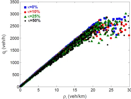
Conventionally, the fundamental relationship is derived from historic measurements, and it also depends on several factors, see [2, 17]. Therefore, the analysis on the mixed traf- fic flow requires several experiments with various rates of autonomous vehiclesκ. Figure 2 shows an example of the result of the analysis, which is performed through the VISSIM traffic simulator. It can be seen that the increase inκ(k)has the following effects on the linear section (ρ_i(k) ∈ [0;ρ_i,crit]) of the fundamental characteristics, whereρ_i,crit is the density value at the maximum ofq_i(k).

• Through the increase inκ(k) the mean value of the traffic flow characteristics de- creases. The decrease has a progressive tendency.

• Similarly, the increase inκ(k)leads to the increase in the density in the set of traffic flow values. The increase in density is also nonlinear.

The experiments of the simulations on the linear section of the fundamental diagram are formulated in the following relationship

q_i(k) = α₀−f_β(κ(k))

ρ_i(k) +f_γ(κ(k))ρ_i∆_i

= (α0−(β2κ²(k) +β1κ(k)))ρi(k)+

+ (γ3κ³(k) +γ2κ²(k) +γ1κ(k) +γ0)ρi∆_i, (4) wherefβ, fγ areκ(k)-dependent polynomial functions of the model with the parameters α0, β2, β1andγ3, γ2, γ1, γ0. ∆i ∈ [−1; 1]represents the uncertainty in the system, which results in the density in the flow characteristics.

The traffic flow model of a freeway sectioniis formed through the law of conservation

Figure 2: Charactersitics of the fundamental diagram

(1) and the proposed form of the fundamental relationship (4) ρ_i(k+ 1) =ρ_i(k) + T

L_i

qi−1(k) +r_i(k)−s_i(k)−

− (α₀−f_β(κ(k)))ρ_i(k) +f_γ(κ(k))ρ_i∆_i

(5) The equation can be transformed into a state-space representation as

x(k+ 1) =A(κ)x(k) +B1w(k) +B2u(k), (6)

where x(k) = ρi(k) is the state of the system, u(k) = ri(k) is the control input and w(k) =

qi−1(k) si(k) ∆i(k)T

is the disturbance vector. The matrix of the system is represented byA, and simultaneouslyB₁ is the matrix of the disturbances and B₂ is the matrix of the control input, such as

A(κ) =

1− T L_i

α0−f_β(κ(k))

, (7a)

B₁ =h

T Li −_L^T

i −_L^T

ifγ(κ(k))ρi

i, (7b)

B2 = hT

Li

i

. (7c)

3 Design of LPV control for the traffic flow

The purpose of this section is to find a control method by which the controlled inflow of the freeway rampri(k)is set, while the control input is limited and the impact of disturbances must be eliminated. Moreover, a challenge in the control design is that the dynamics of the traffic is modeled in an LPV form, see (6).

The aim of the control is to guarantee the maximum outflow q_i(k) of the traffic net- work. However, the outflow can be improved by increasingρi(k)until reaching the critical densityρi,crit. Sinceqi(k)has a maximum atρi,crit[18], it must be guaranteed through the coordination of the system inputs:

z1 =ρi,crit−ρi(k), |z1| →min, (8)

Although at a low number of inflow vehiclesρi,critcannot be achieved, but increasingρi(k) throughz1 results in the maximization ofqi(k). The value of critical density is selected through the previous analysis of the traffic network.

The design of the control requires several steps to find an appropriate controller on the existing complex problem. Thus, the following steps must be performed in the method.

1. The constraint on the control input is considered in the design method.

2. The traffic model through the consideration of (8) is reformulated.

3. The LPV system is described in a Takagi-Sugeno form, which leads to a linear control design problem.

4. The control synthesis is formed as an optimization problem, in which the impact of the disturbances on the performance is reduced.

3.1 Consideration of the input constraints

In the traffic system the value of control inputr_i(k)must be non-negative. Moreover, the inflow on the ramps can have a maximum capacity due to the physical limits of the road.

Thus, it is necessary to design a control strategy, by which the following constraint is han- dled

0≤r_i(k)≤r_i,max, (9)

whereri,max represents the maximum capacity of the inflow ramps. The criterion is con- sidered as a soft constraint during the control actuation in the following way.

It is necessary to consider that the control intervention has importance at highρivalues, which are close toρ_i,crit. Ifρ_i is significantly smaller thanρ_i,crit,r_i =r_i,max is selected.

This intervention is operated in the range of0 ≤ρ_i(k)≤ρ_i,des, whereρ_i,des < ρ_i,critis a design parameter.

However, ifρ_i > ρ_i,des, the value ofr_i must be reduced to avoid the saturation of the traffic network. In this case the dynamic control must be actuated, whose design is based on the control-oriented traffic model. The model (6) in the range of ρ_i > ρ_i,des must be reformulated to eliminate the static density value ofρ_i,desin the control design. The model (6) atx(k+ 1) =x(k) =ρi,desis formed as

ρi,des =A(κ)ρi,des+B1wst+B2ust, (10)

wherew_stis considered to be an average disturbance atρ_i,desandu_st is the related control input, which is computed as

u_st =B⁻¹₂

(1−A(κ))ρ_i,des−B₁w_st

. (11)

Moreover, the avoidance of the saturation requires a dynamic actuation u_dyn(k), which guarantees the performance (8) and reduces the impact of wdyn(k) on the performance.

w_dyn(k) >0is considered to be the difference betweenw(k)andwst. Thus, the control- oriented traffic model (6) for the control design on the range ofρ_i,des ≤ ρ_i(k) ≤ρ_i,crit is reformulated as

x_dyn(k+ 1) =A(κ)x_dyn(k) +B₁w_dyn(k) +B₂u_dyn(k), (12) wherex_dyn(k) =x(k)−ρ_des,i. Simultaneously, the overall control actuation is

ri(k) =u(k) =ust+u_dyn(k), (13)

from which the constraints ofudyn(k)is

−ust ≤udyn(k)≤ri,max−ust. (14)

The main result of the reformulation is that the dynamic control inputu_dyncan have both positive and negative values, see (14), with which the complexity of the control design can be significantly reduced. However, the overall control input on the traffic systemu(k) is always non-negative.

3.2 Performance-driven reformulation of the traffic model

The goal of the control design is to guarantee the defined performance (8). Thus, it is necessary to minimize the difference between the current traffic density and the critical density value. Due to the partition of the system into static and dynamic parts, performance z1 is modified to

e(k) =ρ_ref −x_dyn(k), |e(k)| →min, (15) whereρ_ref =ρ_i,crit−ρ_i,desis a constant value.

The error fork+ 1is derived ase(k+ 1) =ρref−xdyn(k+ 1). Using the relationship (12), the dynamics of the error is

e(k+ 1) =ρref−A(κ)xdyn(k)−B1wdyn(k)−B2udyn(k) =

=ρref −A(κ)(ρref −e(k))−B1wdyn(k)−B2udyn(k) =

=A(κ)e(k) + (1−A(κ))ρ_ref −B₁w_dyn(k)−B₂u_dyn(k). (16) The controller of the traffic system is considered to be full-state feedback, whose input is e(k). Thus, the control law isudyn=Ke(k), whereKrepresents the controller. Using the relationship betweenu_dynande(k), the error dynamics is formed as

e(k+ 1) = A(κ)−B2K

e(k) +W(k) =Acl(κ, K)e(k) +W d(k), (17) whereW d(k)is an upper-bound approximation of the overall disturbance(1−A(κ))ρref− B1wdyn(k), in which||d(k)|| ≤ 1is a noise andW represents its scaling. The formulated system on the tracking error (17) is an LPV system, in whichKmust be selected to stabilize the system, guarantee the performances and reduce the impact ofd(k)one(k).

3.3 Takagi-Sugeno description of the system

In the following the LPV system (17) is reformulated to the sum of Linear Time Invariant (LTI) systems using the Takagi-Sugeno description, see [10]. The advantage of the method is that the control design becomes simpler due to the linear formulation.

The scheduling variable κ has lower κ and upper κ limits. Similarly, the limits de- termine the lower and upper limits of Acl(κ, K), such as Acl = Acl(κ, K) andAcl = A_cl(κ, K). Thus,A_cl(κ, K)can be reformulated as

A_cl(κ, K) = Acl−Acl

Acl−Acl

A_cl+A_cl−A_cl Acl−Acl

A_cl =µ₁A_cl+µ₂A_cl, (18) where0 ≤ µ1, µ2 ≤ 1are the multipliers of the matricesAcl, Acl. Similarly, the system (17) can be reformulated using (18) as

e(k+ 1) =µ1(Acle(k) +W d(k)) +µ2(Acle(k) +W d(k)), (19) which means that the original LPV system can be reformulated as a sum of two linear systems, which represent the convex hull of theκ-dependent LPV system.

3.4 Synthesis of the optimal control

During the control synthesis it is necessary to guarantee the stability of the system and the improvement of the performances. In addition, the impact of the disturbances on the tracking must be reduced. These criteria are formed in the following way.

• Stability: For the stability of the set of LTI systems (19) it is necessary to guarantee that all trajectories of the systems converge to zero as t → ∞ [14]. Thus, it is necessary to guarantee the stability criterion

∆V(e(k))<0, (20)

whereV(e(k)) >0is the Lyapunov function. ∆V(e(k))is selected in a quadratic form, such asV(e(k)) = e(k)^TP e(k), P > 0andP is a symmetric matrix. The stability criterion for the systemA_cle(k) +W d(k)is derived as

∆V(e(k)) =V(e(k+ 1))−V(e(k)) =

= (Acle(k) +W d(k))^TP(Acle(k) +W d(k))−e(k)^TP e(k) =

=e^T(k)(A^T_clP Acl−P)e(k) +e^T(k)A^T_clP W d(k) +W^Td^T(k)P Acle(k)+

+W^Td^T(k)P W d(k) = e(k)

d(k) T"

A^T_clP Acl−P A^T_clP W W^TP^TA_cl W^TP W

# e(k) d(k)

<0.

(21) The result of the derivation can be formed as a Linear Matrix Inequality (LMI) con- dition on systemAcle(k) +W d(k), such as

"

A^T_clP Acl−P A^T_clP W W^TP^TA_cl W^TP W

#

≺0. (22)

Similarly, the LMI condition for systemA_cle(k) +W d(k)is A^T_clP A_cl−P A^T_clP W

W^TP^TA_cl W^TP W

≺0. (23)

SinceA_cl, A_cldepend on the controllerK, it is necessary to selectKandP >0, by which the previous conditions are guaranteed.

• Performance: The tracking capability of the system (8) can be improved through the selection ofK. Since the control input is defined asu_dyn(k) =Ke(k), the tracking can be improved by increasing the gainK.

• Disturbance: The reduction of the impact ofd(k)one(k)requires that theH_∞norm of the transfer functionT_d,efromd(k)toe(k)be reduced. In the systemA_cle(k) + W d(k)the transfer function is computed as

T_d,e= zI−A_cl−1

W, (24)

whereIis an identity matrix. Thus, the condition is

||T_d,e||_∞=

zI−A_cl−1

W

_∞< γ, (25)

whereγ > 0is a predefined upper bound of the norm. Ifγ < 1is selected then the robustness of the system can be guaranteed, see [19]. Similarly, the criterion on the systemA_cle(k) +W d(k)is

zI−A_cl−1

W

∞< γ. (26)

The conditions of (25) and (26) can be composed with the criteria (22) and (23) through the dissipativity of the system, the construction of the supply function and the Schur lemma, see [14]. Thus, the LMI conditions which incorporate the stability and the distrubance rejection criteria are









P 0 A^T_clP I 0 γ²I W^TP 0 P A_cl P W P 0

I 0 0 I









0, (27a)









P 0 A^T_clP I 0 γ²I W^TP 0 P A_cl P W P 0

I 0 0 I









0. (27b)

During the control synthesis it is necessary to minimize γ, while K is maximized.

Therefore, during the optimization ¹_γ in a cost function

J =K+αγ (28)

is maximized, whereαis a scaling parameter. Thus, the resulting optimal control problem is

maxK,γ K+αγ (29a)

subject to P 0, (29b)

where









P 0 A^T_clP I 0 γ²I W^TP 0 P A_cl P W P 0

I 0 0 I









0, (30a)









P 0 A^T_clP I 0 γ²I W^TP 0 P Acl P W P 0

I 0 0 I









0. (30b)

The resulting optimal controllerK is used to computeu_dyn, which is applied as a con- trol input to the system together with theust.

4 Simulation example

In the following a simulation example on the robust LPV control is presented. In the simula- tion a1.5-km-long section of the Hungarian M1 freeway between Tatab´anya and Budapest with two lanes is examined. Previously, several simulations have been performed in the VISSIM traffic simulator to generate the fundamental characteristics of the freeway. Dur- ing these simulations several traffic scenarios with variousκandq0values were performed.

Some preliminary results can be found in [20]. During the simulations it was observed that ρ_crit was around25veh/km, which resulted in the setting ofρ_des = 22veh/km.

In the simulation the freeway section has two inflows. First, q0 is the uncontrolled inflow from the previous highway section. Second, the traffic system has one controlled ramp with inflowu. The controlled gate is located at the beginning of the freeway section.

Moreover, the vehicles can leave the freeway section on an outflow ramps1 and they can also transfer to the next freeway section with the flowq1. During the simulation the ratio of the autonomous vehiclesκcontinuously varies. In the traffic model the freeway section is handled as one segment, thusi≡1.

Figure 3 illustrates the disturbances of the system, which areq0 ands1. These signals cannot be influenced through the designed control, but the role of the control strategy is to guarantee the maximum outflow and reduce the impact of disturbances on it. It can be seen that the currentq0oscillates around1800veh/h, which can result in a high value forρ1

together withr₁, see e.g. att= 1000s q₀ = 2100veh/km, which yieldsρ₁ = 28veh/km.

Thus, it is necessary to limit the inflow of the vehicles on the inflow ramp. Moreover,s1has a small value, which means that most of the vehicles along the freeway section are driven.

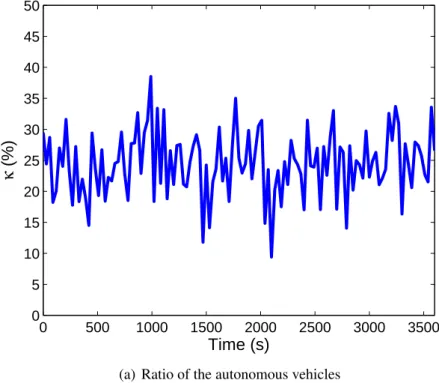
The ratio of the autonomous vehicles in the heterogeneous traffic is shown in Figure 4(a). During the simulation it varies between10%. . .40%, which is a significant variation.

Moreover, the resulting densityρ1 can be seen in Figure 4(b). The results show that the requiredρ_crit = 25 veh/km is tracked by the controlled system with low error, which provides maximum outflow.

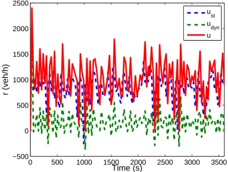
Finally, the control input and its components are illustrated in Figure 5. The control inputu_sthas a higher value, with which the constraint onr₁is guaranteed. Moreover,u_dyn guarantees low error in the tracking. The efficiency of the control can be illustrated at time t = 1000 s. In this case the freeway section has a high load on q0, which can lead to a congestion. Thus, the control inputu is significantly reduced with componentsu_st and u_dyn, see Figure 5. Throughout simulation the overall control inputu = u_st +u_dyn has

0 500 1000 1500 2000 2500 3000 3500 1400

1500 1600 1700 1800 1900 2000 2100 2200

Time (s) q 0 (veh/h)

(a) Uncontrolled inflow on the freeway

0 500 1000 1500 2000 2500 3000 3500 50

60 70 80 90 100 110 120 130 140 150

Time (s) s 1 (veh/h)

(b) Outflow on the ramps

Figure 3: Disturbances in the simulation

a value between0. . .2450veh/h, whose mean is 1100veh/h. As a result the mean of the entire inflow of the sectionq0 +r1 is2900veh/h. In spite of the high inflow and the varyingκ performance is guaranteed, which proves that the LPV-based control strategy is suitable for the solution of the traffic control problem.

0 500 1000 1500 2000 2500 3000 3500 0

5 10 15 20 25 30 35 40 45 50

Time (s)

κ (%)

(a) Ratio of the autonomous vehicles

0 500 1000 1500 2000 2500 3000 3500 15

20 25 30

Time (s) ρ 1 (veh/km)

(b) Traffic density on the section

Figure 4: Simulation results

5 Conclusions

The paper has presented a control strategy for the optimization of heterogeneous traffic flow, which contains conventional human-driven and autonomous vehicles. It has been derived

0 500 1000 1500 2000 2500 3000 3500

−500 0 500 1000 1500 2000 2500

Time (s)

r (veh/h)

ust

udyn

u

Figure 5: Control input in the simulation

from a LPV model for the heterogeneous traffic flow, in which the ratio of the autonomous vehicles is incorporated in a scheduling variable. The robust control design is based on a maximization criterion, which incorporates LMI conditions. Moreover, the control strategy handles the constraints on the control input. The simulation example has illustrated that the proposed robust LPV control is able to guarantee the performance specification of the system, which results in the required traffic density.

Acknowledgement

This work has been supported by the GINOP-2.3.2-15-2016-00002 grant of the Ministry of National Economy of Hungary and the European Commission through the H2020 project EPIC under grant No. 739592.

The work of Bal´azs N´emeth was partially supported by the J´anos Bolyai Research Scholar- ship of the Hungarian Academy of Sciences and the ´UNKP-19-4 New National Excellence Program of the Ministry for Innovation and Technology.

References

[1] B. N´emeth and P. G´asp´ar, “The relationship between the traffic flow and the look- ahead cruise control,” IEEE Transactions on Intelligent Transportation Systems, vol. 18, no. 5, pp. 1154–1164, May 2017.

[2] A. Messmer and M. Papageorgiou, “Metanet - a macroscopic simulation program for motorway networks,”Traffic Engineering and Control, vol. 31, pp. 466–470, 1990.

[3] J. R. D. Frejo, E. F. Camacho, and R. Horowitz, “A parameter identification algo- rithm for the Metanet model with a limited number of loop detectors,” in51st IEEE Conference on Decision and Control, 2012, pp. 6983–6988.

[4] F. Wageningen-Kessels, H. Lint, K. Vuik, and S. Hoogendoorn, “Genealogy of the traffic flow models,”European Journal on Transportation and Logistics, vol. 4, pp.

445–473, 2015.

[5] W. Schakel, B. Van Arem, and B. Netten, “Effects of cooperative adaptive cruise con- trol on traffic flow stability,” in 13th Int. Conference on Intelligent Transportation Systems, 2010, pp. 759–764.

[6] B. Arem, C. Driel, and R. Visser, “The impact of cooperative adaptive cruise con- trol on traffic-flow characteristics,”IEEE Transactions On Intelligent Transportation Systems, vol. 7, no. 4, pp. 429–436, 2006.

[7] A. Bose and P. Ioannou, “Analysis of traffic flow with mixed manual and semi- automated vehicles,”IEEE Transactions on Intelligent Transportation Systems, vol. 4, no. 4, pp. 173–188, 2003.

[8] C. Zhang and A. Vahidi, “Predictive cruise control with probabilistic constraints for eco driving,” inASME Dynamic Systems and Control Conference, vol. 2, 2011, pp.

233–238.

[9] F. Wu, “A generalized LPV system analysis and control synthesis framework,”Inter- national Journal of Control, vol. 74, pp. 745–759, 2001.

[10] P. G´asp´ar, Z. Szab´o, J. Bokor, and B. N´emeth,Robust Control Design for Active Driver Assistance Systems. A Linear-Parameter-Varying Approach. Springer Verlag, 2017.

[11] R. Wiedemann, “Simulation des Strassenverkehrsflusses,”Schriftenreihe des Instituts f¨ur Verkehrswesen der Universit¨at Karlsruhe, vol. 8, 1974.

[12] M. Fellendorf and P. Vortisch,Fundamentals of Traffic Simulation, ser. International Series in Operations Research & Management Science. New York, NY: Springer, 2010, vol. 145, ch. Microscopic Traffic Flow Simulator VISSIM.

[13] S. Boyd, L. E. Ghaoui, E. Feron, and V. Balakrishnan, Linear Matrix Inequalities in System and Control Theory. Philadelphia: Society for Industrial and Applied Mathematics, 1997.

[14] C. Scherer and S. Weiland,Lecture Notes DISC Course on Linear Matrix Inequalities in Control. Delft, Netherlands: Delft University of Technology, 2000.

[15] W. Ashton,The Theory of Traffic Flow. London: Spottiswoode, Ballantyne and Co.

Ltd., 1966.

[16] N. Gartner and P. Wagner, “Analysis of traffic flow characteristics on signalized arte- rials,”Transportation Research Record, vol. 1883, pp. 94–100, 2004.

[17] M. Treiber and A. Kesting, Traffic Flow Dynamics: Data, Models and Simulation.

Berlin,Heidelberg: Springer-Verlag, 2013.

[18] C. Daganzo,Fundamentals of transportation and traffic operations. Oxford: Perga- mon., 1997.

[19] K. Zhou, J. Doyle, and K. Glover,Robust and Optimal Control. Prentice Hall, 1996.

[20] P. G´asp´ar and B. N´emeth, Predictive Cruise Control for Road Vehicles Using Road and Traffic Information. Springer International Publishing, 2019.