Robust H ∞ controller design for T1DM based on relaxed LMI conditions
Gy¨orgy Eigner∗, Istv´an B¨ojthe∗, Alajos M´esz´aros†, Levente Kov´acs∗
∗Physiological Controls Research Center
Research, Innovation and Service Center of ´Obuda University Center, Budapest, Hungary Email: eigner.gyorgy@nik.uni-obuda.hu, bojthez@gmail.com, kovacs@uni-obuda.hu
†Slovak University of Technology in Bratislava
Institute of Information Engineering, Automation and Mathematics, Slovakia Email: alajos.meszaros@stuba.sk
.
Abstract—The aim of this research is to introduce an advanced controller design method which utilizes the Linear Parameter Variable (LPV) and Linear Matrix Inequality (LMI) theorems in order to control a given physiological model related to Diabetes Mellitus (DM). The developed approach is applied on a modified version of the so-called Minimal Model describes Type 1 DM condition. Due to the applied LPV-LMI conditions the resulting controller uses state feedback kind control rule. Further, robust and optimal control requirements have been included during the declaration of LMI rules allowing the formalization of complex requirements. The resulting control structure is robust from the considered disturbances points of view. During the validation we have found that the controller was able to handle highly unfavorable loads beside satisfying the predefined requirements.
Index Terms—Linear Parameter Varying, Nonlinear Systems, Control Engineering
I. INTRODUCTION
Physiological systems do have nonlinear behavior in gen- eral. This phenomena reflects in the properties of mathematical models applied to approximate different behavior of such systems. To apply control on them nonlinear methodologies are needed or such solutions which exploit the properties of specific methodologies in order to control nonlinear systems by avoiding the use of nonlinear control tools [1]–[3].
One of the mostly applied tool of nonlinear control is the adaptation of the methods of Lyapunov introduced originally in [4], [5]. The Lyapunov methods can be applied to inves- tigate the stability of general nonlinear systems. The tools themselves are universal mathematical techniques adaptable for control purposes. From controller design point of view Lyapunov second method – or the direct method – grants a possibility to determine if a nonlinear system is stable or not, without analytically solving the motions of equations. Another important aspect is that many physiological system models do not have analytical solutions in closed form, and adding to this, the validity of numerical solutions are limited [4], [5].
This project has received funding from the European Research Council (ERC) under the European Union’s Horizon 2020 research and innovation programme (grant agreement No 679681). The authors highly acknowledge the contribution of the Scientific Grant Agency of the Slovak Republic under the grants 1/0112/16 and 1/0403/15.
During the last decade, several solutions have surfaced based on Lyapunov’s framework, with sole purpose of de- veloping generalized solutions for nonlinear control. Some of them require the highly creative thinking of an expert designer, and advanced, high computational capacity mathematical so- lutions (eg. LMI) based optimizations. These solutions can yield possibilities for a robust controller design, taking into consideration several key restrictions, and still perform well.
Another approach can be trough LPV methodology. The main benefit of using the LPV framework is, that it allows the usage of linear controller design approaches, because it ”hides”
the nonlinearities of given systems [6]. However, in most cases, the LPV methodology is combined with Lyapunov’s theorems via LMI framework.
This paper is structured in the following way: first, we introduce the basics of LPV systems; then, we present the LPV controller in LMI framework and the ideas behind it;
afterwards, we demonstrate the developed method on given nonlinear T1DM model; finally, we conclude our work and present the future directions.
II. LPVBASED STATE FEEDBACK CONTROL
A. State feedback control
A possible representation of a given Linear Time Invariant (LTI) system is the state space representation where the system is characterized by itsA∈Rk×kstate,B∈Rk×minput,C∈ Rl×k output and D ∈ Rl×m forward matrices, respectively.
The equation of motion of the given system is described as follows:
x(t)˙ y(t)
=
A B C D
x(t) u(t)
=S x(t)
u(t)
, (1)
whereu(t)∈Rmis the control input,y(t)∈Rlis the output andx(t)∈Rk is the state vectors, respectively.
In case of state feedback control, the control signal can be realized as:
u(t) =−Kx(t) , (2)
where u(t) ∈ Rm is the control input vector, K ∈ Rm×n is the feedback gain matrix. The K can be calculated with different iteration-based methods [7].
Generally, this configuration modifies the open-loopAopen
state matrix into Aclosed = Aopen−BK. The poles of the characteristic equation of the closed loop can be calculated in the following way:
|Iλ−A−BK|= 0 (3) and the closed loop poles λclosed fulfill the stability require- ments (or with other words they are Hurwitz) [7], [8].
B. Introduction to LPV systems
Definition 1 - a qLPV model in its state space(SS) form:
Considering a quasi-LPV model described in its state space representation, the compact form of it is expressed in equation 4a by also considering the system disturbance as well:
˙
x(t) =A(p(t))·x(t) +B(p(t))·u(t) +E(p(t))·d(t) y(t) =C(p(t))·x(t) +D(p(t))·u(t) +D2(p(t))·d(t)
(4a) S(p(t)) =
A(p(t)) B(p(t) E(p(t)) C(p(t)) D(p(t) D2(p(t))
, (4b) .
The D2(p(t)) ∈ Rl×h is the disturbance input forward matrix andE(p(t))∈Rk×hdescribes the disturbance as input matrix. Furthermore,p(t)∈Ω∈RN is the so-called time de- pendent parameter vector. In 4a-4b, the matrices introduced in (7) do havep(t)dependency. TheS(p(t))∈R(k+l)×(k+m+h)
represents the parameter dependent resulting system matrix consists of the given system matrices which equivocally con- cludes the qLPV system. Additionally, the p(t)∈Ω∈RN is the parameter vector which is time dependent.
Definition 2 - TheΩ transformational space is the specif- ically confined hyperspace with N dimensions, or the so called hypercube, is factored by the scheduling parameters, more exactly both its minimum and maximum values, as the elements of the parameter vectorp(t):Ω = [p1,min, p1,max]×
[p2,min, p2,max]×...×[pN,min, pN,max]∈RN. C. A modified bounded real lemma based LMI
The H∞ theory became a widely applied tool regarding robust control in the last two decades. The bounded real lemma (BRL) allows to transfer the H∞ robust control prob- lem into an LMI problem through which the H∞ problem is solved by using LMI based numerical optimization. The lemma can be applied for LPV systems as well, however, it’s conservativeness has only been relaxed in the recent times [9]. By using the findings of [9] a state feedback kind controller gain can be designed which is able to guarantee the robust performance and other prescriptions for LPV systems, however, the gain itself is not parameter dependent. The (5) presents the LMI structure which need to be solved through iterative optimization in order to get one feedback gain which can be used in case of any parameter condition related to
the applied LPV model [9]. The LMI for that purpose is the following:
minimize
M,Q,P γ subject to Pi>0 r >0
AiQ+QTATi +B2iM+MTBT2i Pi−Q+rAiQ+rMTBT2i Pi−Q+rQTAT+rB2iM −r(Q+QT)
CiQ+D2iM rCiQ+rD2iM
BT1i 0
QTCTi +MTDT2i B1i
rQTCTi +rMTDT2i 0
−I D1i
DT1i −γ2I
,
(5) wherei= 1, .., N.
The (5) LMI realized the BRL in a more relaxed way compared to original descriptions [9].
In case of (5) the feedback gain which is able to satisfy the prescribed LMI conditions in case of LPV system can be calculated by:
F=MQ−1 (6)
III. THE USED MODEL AND ITS STATES
A. The extended minimal model
The applied model consists of different submodels. The core is the minimal model describing the glucose-insulin dynamics [10] ((7e)-(7g)), while the CHO and insulin ab- sorption submodels are coming from [11] ((7a)-(7d)). The application of mixed models are frequent in the scientific literature [12]–[14]. The CHO and insulin sub-models have been proposed by Hovorka et al. originally in [11], [15].
Both sub-models are two compartmental models. The CHO submodel describes how the orally ingested CHO affects the rate of appearance of glucose in blood. The insulin absorption submodel describes the rate of appearance of insulin in the blood injected subcutaneously. The submodels are represented by (7a) - (7d). The core model – appeared in [10] – responsible to describe the glucose-insulin dynamics (7e) - (7g).
D˙1(t) =− 1
τDD1(t) + 1000Ag
MwGVGC·d(t) (7a) D˙2(t) =− 1
τD
D2(t) + 1 τD
D1(t) (7b)
S˙1(t) =− 1 τS
S1(t) + 1 VI
u(t) (7c)
S˙2(t) =−1
τSS2(t) + 1
τSS1(t) (7d)
G(t) =˙ −(p1+X(t))G(t) +p1GB+ 1 τD
D2(t) (7e)
X˙(t) =−p2X(t) +p3(I(t)−IB) (7f)
I(t) =˙ −n(I(t)−IB) + 1 τS
S2(t) (7g)
The core model has three state variables, which are con- nected to the blood plasma, these are:G(t)[mg/dL] the blood glucose (BG) concentration, X(t) [1/min] insulin-excitable tissue glucose uptake activity, I(t) [mU/L] the blood insulin concentration. The glucose and insulin absorption submodels consist of the D1(t) [mg/dL],D2(t)[mg/dL], S1(t)[mU/L]
and S2(t) [mU/L], respectively. The disturbance input d(t) [g/min] represents the glucose intake which is transformed by the (1000Ag)/(MwGVG)
Ccomplex into the appropriate di- mension to fit to theD1(t). The control inputu(t)[mU/L/min]
is directly connected to theS1(t). The detailed description of the used model parameters can be found in Table??.
Table I
THE APPLIED PARAMETERS OF THE MODELS[10], [11].
Notation Value Unit Description
GB 110 [mg/dL] Basal glucose level
IB 1.5 [mU/L] Basal insulin level
p1 0.028 [1/min] Transfer rate
p2 0.025 [1/min] Transfer rate
p3 0.00013 [L/(mU min)] Transfer rate
n 0.23 [1/min] Time constant for in-
sulin disappearance
BW 75 [kg] Body weight
VI 0.12BW [L] Insulin distribu-
tion volume
VG 0.16BW [L] Glucose distribu-
tion volume MwG 180.1558 [g/mol] Molecular weight
of glucose
Ag 0.8 - Glucose utilization
C 18.018 [mmol/L]
Convert rate
between [mg/dL]
and [mmol/L]
τD 40 [min] CHO to glucose ab-
sorption constant
τS 55 [min]
Insulin absorption constant
The parameters shown in Table I above are the nominal parameters applied at the controller design process [10].
B. Design of the Extended Kalman Fiter
Due to the only output isG(t)in case of state feedback kind designs, estimation of other states are needed. In this particular case we decided to apply a discrete Extended Kalman Filter (EKF) which is need to handle the nonlinear behavior of the model [16].
In the EKF design the following nonlinear system and noisy observation model is considered:
xk=f(xk−1,uk) +wk
zk =h(xk) +vk
, (8)
where Table II introduces the terms in 8.
Table II
VARIABLES AND FUNCTIONS RELATED TO THE APPLIEDEKF
xk n x 1 state vector
zk m x 1 observation vector
wk n x 1 process noise vector vk m x 1 measurement noise vector f() n x 1 nonlinear vector function of the process h() m x 1 nonlinear vector function of the observation
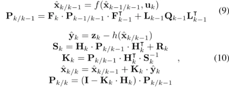
The x0 is considered as an initial state, a vector with a µ0=E[x0]and a covariance ofP0=E[(x0−µ0)·(x0−µ0)|] and uk is the control vector. The f function’s task is state prediction based upon the previous estimate, while functionh gives a predicted measurement from that previously predicted state. The prediction and update phases are described by (9) - (10) [16].
ˆ
xk/k−1=f(ˆxk−1/k−1,uk)
Pk/k−1=Fk·Pk−1/k−1·F|k−1+Lk−1Qk−1L|k−1 (9) ˆ
yk =zk−h(ˆxk/k−1) Sk=Hk·Pk/k−1·H|k+Rk
Kk=Pk/k−1·H|k·S−1k ˆ
xk/k = ˆxk/k−1+Kk·yˆk Pk/k= (I−Kk·Hk)·Pk/k−1
, (10)
whereIis the unit matrix in appropriate dimensions.
The prediction phase is presented in equation (9), firstly the state estimate and after that, the estimated covariance is predicted. In equation (10) the updating stage is presented. The ˆ
yrepresents the measurement residual, whileSk is the resid- ual covariance, this is used to calculate an optimal Kalman gain (Kk) so that the state estimate (ˆxk/k) and covariance estimate (Pk/k) can be updated. The state transition (Fk) and observation (Hk) are represented by the following Jacobian matrixes [16]:
Fk = ∂f∂x|ˆxk−1/k−1,uk
Hk =∂h∂x|ˆxk/k−1 (11) IV. CONTROLLER DESIGN
Due to the state feedback kind controller applied in this study the use of difference based control oriented model form is beneficial. In this case reference compensation is not need to be designed. The transformed model represents the error dynamics, namely the deviation of state variables of the transformed model from a given equilibrium. Thus, when the state feedback kind controller forces the decay of the trans- formed state variables it basically coerces the state variables of the original system to converge the given equilibrium. In this particular case the applicable formalism is the following:
∆x(t) =x(t)−x1,ref and∆u(t) =u(t)−uref(t)instead of the states from (4a)-(4b). These new states form the dynamics of error and let to use ther=02×1 reference signal. Hence
∆x(t)→0, while t → ∞. The transformation of the states can be done as it is detailed in 12 in case of (7a)-(7g) as well.
∆ ˙G(t) = ˙G(t)−0 =
−p1G(t)−X(t)(G(t) +Gb) +d(t)−
−p1Gref−Xref(Gref+Gb) +href
=
−p1∆G(t) + ∆d(t)−Gb∆X(t)−X(t)G(t) +XrefGref
+XrefG(t)−XrefG(t)
∆ ˙G(t) =−(p1+Xref)∆G(t)−G(t)∆X(t) + ∆d(t)
(12)
.
The transformations are similar in case of other state vari- ables as well.
To adapt the (4a)-(4b) to our case and extend it we applied the following modification. The first two equations were al- ready mentioned in (4a) as describing an LPV system, the third equation below – refers to z(t) – represents the performance output:
∆ ˙x(t) =A(p(t))·∆x(t) +B(p(t))·∆u(t)+
E(p(t))·∆d(t)
∆y(t) =C(p(t))·∆x(t) +D(p(t))·∆u(t)+
D2(p(t))·∆d(t)
∆z(t) =C2,∞(p(t))·∆x(t) +D2,∞(p(t))·∆u(t)+
E2,∞(p(t))·∆d(t)
(13) where C2,∞(p(t)) ∈ Rq×m, D2,∞(p(t)) ∈ Rq×m and E2,∞(p(t)) ∈ Rq×h. In this study we have considered that the input, output and performance related matrices are not parameter dependent, also do have constant values. Hence, th following system obtains in the form of (13):
S(p(t)) =
A(p(t)) B E
C D D2
C2,∞ D2,∞ E2,∞
=
=
− 1
τD 0 0 0 0
1 τD
− 1 τD
0 0 0
0 0 −1
τS
0 0
0 0 1
τS
−1 τS
0
0 1
τD
0 0 −(p1+Xref)
0 0 0 0 0
0 0 0 1
τS
0
0 0 0 0 1
0 0 0 0 1
0 0 0 1000Ag
MwGVG
C
0 0 0 0
0 0 1
VI
0
0 0 0 0
−G(t) 0 0 0
−p2 p3 0 0
0 −n 0 0
0 0 0 0
0 0 d2,∞ 0
(14)
.
Thed2,∞is applied as a scaling parameter determining the weight of the control signal’s effect in the performance output.
The (IV) has applied during the optimization process of (5) in order to get oneFcontroller gain.
We have investigate four scenarios, however. The scenarios have been the following:
1) Thep(t) =G(t)andp= [70, ...,300].
2) The p(t) = G(t) and pI = [70, ...,120] and pII = [120, ...,300]. The parameter domain have been divided into two parts and two FI,II has been designed for the two subdomains.
3) Thep(t) = [G(t), p1(t)]> andp1= [70, ...,300].
4) The p(t) = [G(t), p1(t)]> and p1,I = [70, ...,120]
and p1,II = [120, ...,300]. The G(t) related parameter domain has been divided into two parts and two FI,II
have been designed for the two subdomains.
With d2,∞ the scale of the control signal can be managed and reduced. Trough this LMI, it is possible to minimize the control signal while designing a robust controller. In the performance output, it is taken into consideration, to have as good disturbance suppression as possible, but also to have as small control signal as possible. This double criteria could be realized with the chosen LMI parameters. Moreover, these restrictions are applied on the difference based model which allow us to define interpret them to ”as small difference from a given BG level as possible” and ”as small control signal from the a given level as possible”.
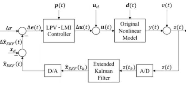
Figure 1 shows the control structure of the complete TP- LMI-LPV system.
Figure 1. The control system
V. RESULTS
In the following examples a normal daily eating routine of a human is taken as disturbance. Breakfast, lunch and dinner serve as the main calorie intakes, in between them, there are two smaller meals consumed, serving as snacks.
The disturbance for the system in each scenario is the same and can be seen on figure 2. Numerically, it is 250 grams of carbohydrate from which 210 g is divided in three making up the three main meals of the day while the remaining 40 g is divided in two serving as the snacks.
In the following four figures, the results of the four control scenarios are displayed. Each figure has three separate sub- figures incorporated one over the other, these represent the model states with the blood glucose level highlighted and the input signal respectively. For the controller design and calculation of the feedback gains, MOSEK Apps. solver [17]
and the YALMIP toolbox [18] were used.
T ime [hour]
0 5 10 15 20
Carbohydrateintake[g]
0 2 4 6 8 10 12 14 16 18 20
Figure 2. The applied glucose intake as disturbance
T ime [hour]
0 5 10 15 20 25
Systemstates
-200 0 200 400 600
D1 D2 S1 S2 G X I T ime [hour]
0 5 10 15 20 25
BloodGlucoseLevel[mg/dL]
50 100 150 200
T [hour]
0 5 10 15 20 25
Controlsignal
0 50 100 150
Figure 3. Results for scenario 1
In the first scenario, the only variable parameter is Gand the domain is not split into two parts, namely,G= [70,300].
The parameters of the LMIs shown in the previous section were: γ = 38.72 and d2,∞ = 0.97, r = 0.35. The lowest value it got, with this controller was 70.0270 [mg/dL]. The following feedback gain occured, as it can be seen in equation (15):
F=
0.0003 0.0004 −0.0002 −0.0004
−0.0004 −2.0476 −0.0001
·103 . (15) In the second scenario the parameter domain was divided in two, and a standalone controller was designed for both partitions, arguably a more robust controller can be obtained en-bloc this way. The first partition of G is between 70and 120 and naturally, the second one is[120,300]. Two different controllers were designed with different feedback gains (FI andFII, equations 16 and 17 respectively) for the partitions, with differing parameters for the LMIs. The LMI parame-
T ime [hour]
0 5 10 15 20 25
Systemstates
-200 0 200 400 600
D1 D2 S1 S2 G X I T ime [hour]
0 5 10 15 20 25
BloodGlucoseLevel[mg/dL]
50 100 150 200
T [hour]
0 5 10 15 20 25
Controlsignal
0 50 100 150
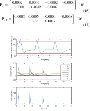
Figure 4. Results for scenario 2
ters concerning the first controller were: d2,∞ = 0.6555, γ= 23.45andr= 0.30. The LMI parameters concerning the second controller were:d2,∞= 1.2,γ= 37.41andr= 0.35.
The lowest value it reached, with this controller is 70.0708 [mg/dL].
FI =
0.0002 0.0004 −0.0002 −0.0004
−0.0008 −1.4042 −0.0007
·103 . (16) FII =
0.0003 0.0005 −0.0004 −0.0008 0 −3.35 −0.0017
·103 . (17)
T ime [hour]
0 5 10 15 20 25 30 35
Systemstates
-200 0 200 400 600
D1 D2 S1 S2 G X I T ime [hour]
0 5 10 15 20 25
BloodGlucoseLevel[mg/dL]
50 100 150 200
T [hour]
0 5 10 15 20 25 30 35
Controlsignal
0 50 100 150
Figure 5. Results for scenario 3
In the third scenario, a second system parameter was in- troduced, p1. The parameter domain is a bounded hypercube equal to G= [70,300]andp1 = [0.0050.1]. The parameters concerning the LMIs were:γ= 114andd2,∞= 2.5,r= 2.2.
The lowest value it reached, with this controller was70.3781 [mg/dL]. The following feedback gain occured, as it can be seen in equation 18:
F=
0.0002 0.0003 −0.0003 −0.0004
−0.0001 −1.1694 −0.0006
·103 . (18)
T ime [hour]
0 5 10 15 20 25
Systemstates
-200 0 200 400 600
D1 D2 S1 S2 G X I T ime [hour]
0 5 10 15 20 25
BloodGlucoseLevel[mg/dL]
50 100 150 200 250
T [hour]
0 5 10 15 20 25
Controlsignal
0 50 100 150
Figure 6. Results for scenario 4
In the fourth scenario, two system parameter-variables were used within a divided domain, the division was the same as seen during the second scenario. The LMI parameters for the first controller were: d2,∞2.6, γ = 89.16 and r = 1.8. The LMI parameters for the second controller were: d2,∞= 5.6, γ = 90.55 and r = 2.7. The lowest value it reached, with this controller was70.0138 [mg/dL]. The following feedback gains occured:
FI =
0.0003 0.0004 −0.0004 −0.0005 0 −1.3396 −0.0007
·103 . (19) FII =
0.0348 0.0424 −0.0815 −0.1096
−0.1340 −306.2058 −0.1670
. (20) VI. CONCLUSION
The goal of this study was the design of an LPV-LMI based state-feedback controller by using the findings of [9] that is as robust as possible in order to map whether the design procedure and application of the relaxed BRL are possible regarding T1DM research. Four steps were taken to obtain a more robust controller, that resulted in four scenarios with
four different results. In either of the scenarios, hypoglycemic values were not registered, but a minor crossing into hyper- glycemic territory was inevitable due to the complexity of the system. It was more relevant to concentrate on avoiding hypoglycemia rather than hyperglycemia because in the short term, only hypoglycemia is deadly the latter only has long term complications. The objectives of stabilizing the blood sugar level at110 [mg/dL]while not reaching hypoglycemic levels (below 70 [mg/dL]) were met. We have found that all of the developed controllers were able to meet with the predefined criteria as it can be seen in Figs 3-6. The BG level have been higher than the critical70 [mg/dL]. We have found that splitting the parameter space into two parts did not provide significant changes in the results.
REFERENCES
[1] J. Bronzino and D. Peterson, Eds.,The Biomedical Engineering Hand- book, 4th ed. Boca Raton, USA: CRC Press, 2016.
[2] T. Ferenci, J. S´api, and L. Kov´acs, “Modelling Tumor Growth Under Angiogenesis In-hibition with Mixed-effects Models,”ACTA Pol Hung, vol. 14, no. 1, 2017.
[3] L. M. Huyett, E. Dassau, H. C. Zisser, and F. J. Doyle III, “Glucose Sensor Dynamics and the Artificial Pancreas: The Impact of Lag on Sensor Measurement and Controller Performance,” IEEE Contr Syst, vol. 38, no. 1, pp. 30–46, 2018.
[4] A. Lyapunov, “A general task about the stability of motion (in russian),”
Ph.D. dissertation, University of Kharkov, Kharokov, Russia, 1892.
[5] ——,Stability of Motion. New York, USA: Academic Press, 1966.
[6] A. White, G. Zhu, and J. Choi,Linear Parameter Varying Control for Engineering Applicaitons, 1st ed. London: Springer, 2013.
[7] R. Burns, Ed.,Advanced Control Engineering, 1st ed. Oxford, UK:
Butterworth-Heinemann, 2001.
[8] W. Levine, Ed.,The Control Engineering Handbook, 2nd ed. Boca Raton, USA: CRC Press, Taylor and Francis Group, 2011.
[9] W. Xie, “An equivalent lmi representation of bounded real lemma for continuous-time systems,”Journal of Inequalities and Applications, vol.
2008, no. 1, p. 672905, 2008.
[10] F. Chee and T. Fernando, Closed-Loop Control of Blood Glucose.
Heidelberg, Germany: Springer, 2007.
[11] R. Hovorka, V. Canonico, L. Chassin, U. Haueter, M. Massi-Benedetti, M. Orsini-Federici, T. Pieber, H. Schaller, L. Schaupp, T. Vering, and W. M.E., “Nonlinear model predictive control of glucose concentration in subjects with type 1 diabetes,”Physiol Meas, vol. 25, no. 4, pp. 905 – 920, 2004.
[12] D. Boiroux, M. Hagdrup, Z. Mahmoudi, K. Poulsen, H. Madsen, and J. B. Jørgensen, “An ensemble nonlinear model predictive control algorithm in an artificial pancreas for people with type 1 diabetes,” in 2016 European Control Conference (ECC). IEEE, 2016, pp. 2115–
2120.
[13] D. Boiroux, A. K. Duun-Henriksen, S. Schmidt, K. Nørgaard, N. K.
Poulsen, H. Madsen, and J. B. Jørgensen, “Adaptive control in an artificial pancreas for people with type 1 diabetes,” Cont Eng Prac, vol. 58, pp. 332–342, 2017.
[14] K. Turksoy and A. Cinar, “Adaptive control of artificial pancreas systems: a review,”J Health Eng, vol. 5, no. 1, pp. 1–22, 2014.
[15] R. Hovorka, F. Shojaee-Moradie, P.V. Carroll, L.J. Chassin, I.J. Gowrie, N.C. Jackson, R.S. Tudor, M. Umpleby, and D.H. Jones, “Partitioning glucose distribution/transport, disposal, and endogenous production dur- ing ivgtt,”Am J Physiol Endocr Metab, vol. 282, no. 5, pp. E992 – 1007, 2002.
[16] M. Grewal and A. Andrews,Kalman Filtering: Theory and Practice Using MATLAB, 3rd ed. Chichester, UK: John Wiley and Sons, 2008.
[17] MOSEK ApS, The MOSEK optimization toolbox for MATLAB manual. Version 7.1 (Revision 28)., 2015. [Online]. Available:
http://docs.mosek.com/7.1/toolbox/index.html
[18] J. L¨ofberg, “YALMIP : A Toolbox for Modeling and Optimization in MATLAB,” in In Proceedings of the CACSD Conference, Taipei, Taiwan, 2004.