Tensor Product Model Transformation based Par- allel Distributed Control of Tumor Growth
Levente Kov´acs and Gy¨orgy Eigner
Physiological Controls Research Center
Research and Innovation Center of ´Obuda University H-1034, Budapest, B´ecsi ´ut 96/B
{kovacs.levente,eigner.gyorgy}@nik.uni-obuda.hu
Abstract: The current work investigates tumor growth control under antiangiogenic targeted molecular therapy by use of Tensor Product (TP) transformation. During the dynamics of the tumor growth we have considered that the tumor volume x1(t)is measurable, while due to the lack of information about the second state x2(t)(the inhibitor level in the serum), we have developed an appropriate Extended Kalman Filter (EKF) to estimate it. We applied different quasi Linear Parameter Varying (qLPV) models during the design of the EKF and the controller. Tensor Product model transformation method completed with Linear Matrix Inequality based optimization have been applied to design the main controller. The reference signals were generated by trajectory tracking kind control based on Inverse Dynamic Control - Proportional Derivate compensator, applied it on the ”simulated” (original) model. We did not consider any state disturbance. However, we have taken into account sensor noise in accordance with the properties of the model.
We have found that all of the control goals have been satisfied with the developed control framework: (i) the tumor volume was lower than 1 mm3 at the end of the therapy; (ii) the developed models have approached each other with good accuracy; (iii) the totally injected inhibitor level was physiologically acceptable.
Keywords: Antiangiogenic Targeted Molecular Tumor Therapy, Tensor Model transforma- tion, Linear Parameter Varying, Linear Matrix Inequality, Parallel Distributed Control
1 Introduction
Targeted Molecular Therapies (TMTs) are advanced tumor therapeutic possibilities which can be used beside the classical treatments (e.g. chemotherapy, radiotherapy, etc.). TMT drugs directly inhibit the specific biochemical pathways used by the different kinds of cancers in order for growing, proliferation and spreading [1, 2].
Hence, by TMTs more personalized treatment can be achieved focusing on the vital phenomena of the tumor and applying specific drugs [3]. The main benefits of TMTs are less damaging to the normal cells, causing less side effects, improving
the efficiency of regular therapies and improving the quality of life of the patients [2]. Among the several types of TMTs the mostly commonly used ones are the apoptosis inducers, gene expression inhibitors, signal transmission inhibitors and anti-angiogenic therapies [3].
Angiogen inhibitors are commonly used in modern medicine by targeting the so- called pro-angiogen factor, the vascular endothelial growth factor (VEGF) that in- dicates the endothelial proliferation leading to the formation of new blood vessels.
The tumors produce VEGF in order to get new blood vessels through which they are able to get the nutrients for further growing. By inhibiting this molecular pathway, the new blood vessels formation phenomena can be decreased causing the ”starva- tion” of the tumor [3–5]. The nature of this process is an excellent therapeutic target to be combined with control engineering methodologies optimizing the drug injec- tion and therapy outcomes [6]. One of the most commonly used TMT drugs in case of angiogen inhibition is bevacizumab which is investigated in this study as well as the parametric identification done by the preparation of the applied model [7].
Similarly to other physiological control applications like diabetes or anesthesia [8–
13] the control of tumor growth is challenging due to several unfavorable effects that should be taken into account. The nonlinear nature of the process completed with cross-effects, parameter and model uncertainties and time-delays increases the difficulty of the problem. Recently, several results appeared in the topic of antian- giogenic TMT control problem [6, 14–18].
The current work investigates the combined applicability of advanced control method- ologies. One of the most promising ones is represented by the LPV framework, a useful technique to apply the well-developed linear control methods on the original nonlinear model without linearizing it [19]. The TP model transformation repre- sents another solution that can be combined with LMI based optimization and can be done on LPV functions as well, making it possible to design TP-LPV-LMI kind controllers [20]. These kind of controllers have many beneficial properties: the pa- rameter uncertainties and the nonlinearities can be embedded into the model mak- ing the designed controller robust against these effects. Furthermore, the control requirements can be formulated as LMIs, which can be taken into account during the design procedure in order to guarantee their satisfaction by the control action.
On the other hand, not all of the state variables of given models are available. One suitable solution to deal with this problem is definitely Kalman-filtering. The Ex- tended Kalman Filter (EKF) represents an estimator designed for nonlinear systems that can be used effectively for highly nonlinear as well [21].
The paper is structured as follows: first, the minimal tumor growth model and the developed qLPV models are introduced. After, the controller design procedure is detailed including the TP model transformation, the LMI based optimization, the EKF design and the development of the reference subsystem. Finally, the results of the numerical simulations are presented, done in MATLAB environment.
2 Tumor Growth Models
2.1 The Examined Tumor Growth Model
The current study focuses on the minimal tumor growth model [22,23]. This second- order model includes two state variables: x1(t)[mm3] for the tumor volume and x2(t)[mg/kg] as the serum inhibitor level:
˙
x1(t) =ax1(t)−bx1(t)x2(t)
˙
x2(t) =−cx2(t) +u(t) . (1)
The control input is represented by the inhibitor intakeu(t)[mg/kg/day], while the output of the model is thex1(t)tumor volume – that is assumed to be measurable.
Three scalar parameters determine the dynamic specificities of the model:a[1/day]
is the tumor growth rate, b [kg/mg/day] is the inhibitor rate and c[1/day] is the inhibitor clearance rate. During our investigations the following dataset has been used: [a,b,c]>= [0.27,0.0074,ln(2)/3.9]>. These values are coming from para- metric identification done on measurements from mice experiments related to C38 colon adenocarcinoma [22].
As a result, the model is a simple mathematical formulation of the phenomena. It is assumed that by using only antiangiogen inhibitor (e.g. bevacizumab [24]) the tumor volume can be maintained and decreased. In the lack of inhibitor, thex1(t) tumor volume grows limitlessly with the dynamics determined bya. The nontrivial equilibrium of the model can be calculated as follows:
0=ax1,∞−bx1,∞x2,∞
0=−cx2,∞+u∞ , (2)
from whichx1,∞andu∞becomes:
x2,∞=a b
, (3a)
u∞=−ca b
. (3b)
Hence,x2,∞andu∞are independent fromx1,∞. It is easy to see thatx2(t) =a/bis needed to keep the tumor volume on a certain level andx2(t)>a/bshould be used to decrease thex1(t). The belonging control signals areu(t) =c·a/bandu(t)>c·a/b, respectively. These requirements have to be taken into account during the controller design.
It should be noted that a lower limit was applied against the tumor volume in all kind of models appearing in this study: min(x1(t)) =min(x1,re f(t)) =min(xˆ1(t)) =10−3 mm3– which is an approximation of the zero level. From the antiangiogenic TMTs point of view this is reasonable since the goal of these kinds of therapies are usually not to eliminate (kill) the tumor itself, but to keep its volume under a certain level [25].
2.2 The Reference Model
As it will be introduced later, the main goal of the control is to enforce the original nonlinear model to behave as a given – beneficiary selected – reference model. As x1(t) can be measured, a simple model was developed with decreasing state trajec- tory:
x1,nom(t) =e(−ξ·t)·x1,re f(t0) , (4)
whereξ is a scalar andtrepresents the time. xre f(t0)is the – known – initial value of the reference model which can be determined by exact measurement (ifx1(t0) = x1,re f(t0)) or estimation (if ˆx1(t0) =x1,re f(t0)). This reference model will be used for trajectory determination during the controller design.
2.3 qLPV Model Development
In conformity with [26–28], the general state-space form of an LPV model is the following:
˙
x(t) =A(p(t))x(t) +B(p(t))u(t) y(t) =C(p(t))x(t) +D(p(t))u(t) S(p(t)) =
A(p(t)) B(p(t)) C(p(t)) D(p(t)) x(t)˙
y(t)
=S(p(t)) x(t)
u(t)
. (5)
The considered vectors and parameter dependent matrices are:x(t)∈Rnstate vec- tor,u(t)∈Rminput vector,y(t)∈Rk output vector,A(p(t))∈Rn×nstate matrix, B(p(t))∈Rn×minput matrix,C(p(t))∈Rk×noutput matrix,D(p(t))∈Rk×mfeed- forward matrix and S(p(t))∈R(n+k)×(n+m) system matrix – the latter one is the so-called LPV function (inasmuch any of the state variables is involved as schedul- ing variable we call it quasi-LPV (qLPV) model and qLPV function [27]). The matrices in (5) are dependent from thep(t)∈ΩR∈RRparameter vector that con- sists of the so-called scheduling variables pi(t), namely,p(t) = [p1(t). . .pR(t)]>. TheΩ= [p1,min,p1,max]×[p2,min,p2,max]×. . .×[pR,min,pR,max]∈RRhypercube – a subspace of theRRreal vector space – is characterized by the extremes of thepi(t).
As it will be seen in the subsequent sections, two different qLPV models have been developed and applied. In order to avoid any misunderstanding, alternative nota- tions for the parameter vectors belonging to the qLPV model were used. In case of Model-Iq(t) =q(t)∈R1, while for Model-II this isp(t)∈R2.
2.3.1 Model-I
We have selected theq(t) =x1(t)as scheduling variable from (1) which leads to the following qLPV model:
˙
x(t) =AI(q(t))x(t) +BIu(t) y(t) =CIx(t)
SI(q(t)) =
AI(q(t)) BI CI DI
=
a −bq(t) 0
0 −c 1
1 0 0
, (6)
where the I subscript is related to Model-I. In this case,BI=BandCI=Care equal to each other due to the lack of specific transformation – we only pointed out one state variable. The selected range forq(t)is{10−3, . . . ,5×105}. The lower boundary is related to the aforementioned limitation against the tumor volume. The upper boundary is in conformity with our previous investigations [6]. Model-I was developed to support the EKF design and application as it will be introduced later.
2.3.2 Model-II
In order to apply state feedback kind controller without reference compensation, a corresponding qLPV model is necessary. The difference based control oriented qLPV models can be a solution for this issue [29]. In this case, the deviation between the states of the model to be controlled and from the states of a given reference system should be modeled, namely, the dynamics of the ”state error”. For the actual problem this means:∆x1(t) =x1(t)−x1,re f(t),∆x2(t) =x2(t)−x2,re f(t)and∆u(t) = u(t)−ure f(t). By this transformation the control goal is transformed as well: instead of reaching a certain value by the state variables the new control goal becomes – reaching zero level by the states over time. Hence, ∆x(t) = [∆x1(t),∆x2(t)]>,
∆x(t)→0,t→∞. In case of a state feedback kind controller this can be obtained, if we use the ∆r=02×1 reference signal and the∆x(t)is compared to this zero reference. The derivation of the transformed differential equations is the following:
∆x˙1(t) =x˙1(t)−x˙1,re f(t) =ax1(t)−bx1(t)x2(t)
− ax1,re f(t)−bx1,re f(t)x2,re f(t)
= a∆x1(t)−bx1(t)x2(t)−bx1,re f(t)x2,re f(t) +0= a∆x1(t)−bx1(t)x2(t)−bx1,re f(t)x2,re f(t)
+bx1(t)x2,re f(t)−bx1(t)x2,re f(t) = (a−bx2,re f(t))∆x1(t)−bx1(t)∆x2(t)
∆x˙2(t) =x˙2(t)−x˙2,re f(t) =−cx2(t) +u(t)− −cx2(t) +u(t)
=
−c∆x2(t) +∆u(t)
. (7)
The state-space form of (7) will be the following:
∆˙x(t) =AII(p(t))∆x(t) +BII∆u(t)
∆y(t) =CII∆x(t) SII(p(t)) =
AII(p(t)) BII CII 0
=
a−bp1(t) −bp2(t) 0
0 −c 1
1 0 0
. (8)
The selected scheduling variables have beenp1(t) =x2,re f(t)∈ {a/b+10−3, . . . ,104} andp2(t) =x1(t)∈ {10−3, . . . ,5×105}at whichp(t) = [p1(t),p2(t)]>. If the goal is to keep the tumor’s level on a certain value, x2=a/b should be reached via u=c·a/b. Consequently, we have approached thea/b bya/b+10−3 in order to increase the numerical stability, further, to keep the controllability of Model-II.
p1,max=104is considered the maximum value which may occur [6], while p2,min andp2,maxare the same as in case ofqdiscussed in Model-I.
3 Control Design
3.1 TP Model Transformation and Control
By TP model transformation it was possible to convert the qLPV function into con- vex polytopic TP model form. The resulting TP model is able to describe the initial qLPV function and through the original nonlinear system with given accuracy. The usability of this tool has been proven several times for highly nonlinear systems (e.g. [20, 30–33]), what the physiological systems are in general [34]. Applying the TP model transformation on the qLPV function of (5), the following finite element convex polytopic TP model is obtained:
x(t)˙ y(t)
=S(p(t)) x(t)
u(t)
S(p(t)) =S R
r=1wr(pr(t)) =S×rw(p(t))
. (9)
The core tensor S ∈RI1×I2×...×IR×(n+k)×(n+m) consists of the Si1,i2,...,iR LTI ver- tices. The wr(pr(t))weighting vector function consists of thewr,ir(pr(t)) (ir= 1...IR)continuous convex weighting functions. The convexity is held, if∀r,i,pr(t): wr,ir(pr(t))∈[0,1]and∀r,pr(t):
Ir
i=1
∑
wr,ir(pr(t)) =1.
Different kinds of convex hulls can be applied during the TP model transformation.
In this study the Minimal Volume Simplex (MVS) convex hull was considered that allows the use of the smallest convex hull insideΩ[35]. However, the TP model approximating the original model inside theΩhypercube with certain accuracy de- pends on the applied sampling resolution inΩ[36]. The practical realization of the TP model transformation can be found in [20, 31, 36, 37].
In case of general state-feedback control, the control signal can be generated in the LPV case as follows [20, 27, 30, 31]:
u(t) =−G(p(t))x(t) , (10)
if the case isr(t) =0n×1– which is in conformity with (8) and the used Model-II. In (10), theG(p(t))∈Rm×nis the parameter dependent controller gain. Consequently, the polytopic convex TP controller becomes:
G(p(t)) =G R
r=1wr(pr(t)) =G×rw(p(t)) . (11)
As a result, theG feedback tensor consisting byGi1,i2,...,iR feedback gain matrices belongs to the givenSi1,i2,...,iR LTI systems. Thewr(pr(t))convex weighting func- tions are the same as in (7). Further derivations, explanations and case studies can be found in [32,35,36,38]. The TP model transformation has been successfully adopted and applied in many technical fields thanks to the continuous improvements in the recent times. New approaches have appeared regarding the computational improve- ments related to TP model transformation [39, 40]. The latest research explored that the LMI based controller design methods are sensitive to the applied convex hulls. Hence, the selection of the applicable convex hull manipulation and the con- vex hull candidate with respect to the LMI based controller design methods is a critical aspect [31, 41–43]. Effective convex hull manipulation techniques are intro- duced in [35, 44, 45]. The application of the TP model based control can be found both in physical control systems [46–59] and it was applied in case of physiological controls as well [60–66]. Many other important control approaches regarding the TP model transformation have been elaborated in [56, 67–74]
3.2 Linear Matrix Inequality based Optimization
In accordance with Lyapunov’s direct method, an ˙x(t) =Ax(t) system is stable if there exists a V(x) =x>Pxpositive definite quadratic Lyapunov function and the ˙V(x) =x>(A>P+PA)xis negative definite, namely,A>P+PA<0andP= P>>0[20, 75]. The ˙x(t) =A(p(t))x(t) +B(p(t))u(t)is the system equation of a general, polytopic system, where the[A(p(t)) B(p(t))] =
R r=1
∑
wr(p)[Ar Br]are the polytopic vertices andwr(p)is the belonging convex weighting function [20]. By utilizing theV(x(t)) =x>Px=x>X−1xLyapunov function, the controller candidate becomes [36]:
u(t) =M(p(t))X−1x(t) =
J
∑
j=1wj(p)MjX−1x(t) . (12)
By realizing the derivative of the Lyapunov function, the following term appears, where ”Sym” acronym means symmetric:
V˙(x(t)) =x>(t)X−1·Sym A(p)X+B(p)M(p)
·X−1x>(t) , (13)
The symmetric term can be described by using the polytopic weighting functions as follows:
Sym A(p)X+B(p)M(p)
=
R i=1
∑
R
∑
j=1wi(p)wj(p)Sym AiX+BiMj
<0 . (14)
TheS(p(t)) =Co(S1,S2, . . . ,SR)andG(p(t)) =Co(G1,G2, . . . ,GR)are polytopic structures – the ”Co” acronym means convex combination. In this study, we have applied Parallel Distributed Compensation (PDC) type control. This is possible if the same w(p(t)) weighting functions are used (to describe the polytopic qLPV system and the controller) citeBaranyi:2013. As a result, LMI optimization can be used in order to design a quadratically stabilizing PDC for continuous polytopic systems [75]:
X>0,
−XA>i −AiX+M>i B>i +BiMi>0,
−XA>i −AiX−XA>j −AjX+M>jB>i +BiMj+M>i B>j +BjMi≥0, i< j≤R s.t. ∀p(t):wi(p(t))wj(p(t)) =0,
(15)
whereXn×nis a positive definite and symmetric matrix,Mm×ni is the supplementary matrix andwiandwjare general polytopic weighting functions, respectively.
In accordance with [36, 75], the control gain is calculated as follows: Mi=GiX, thus,Gi=MiX−1. As the level of injectable inhibitor level is limited – in conjunc- tion with the physiological reality – an LMI constraint was applied on the control input to avoid the unrealistically high injections from the drug.
minX,Mµ X≥I, X M>
M µ2I
≥0
. (16)
By using (16), the ku(t)k2≤µ att ≥0 can be guaranteed. This is true ifx(0) lies in the polytope, which needs thatkx(t0)k2≤1, as it is stated in [76]. We have considered the Model-II from (8) during the controller design via LMI optimization.
Due to the constraint onp1,min, the rank(C(AII(p(t)),BII)) =n=2∀p(t), namely, the controllability property of Model-II can be kept in theΩparameter domain.
3.3 Extended Kalman Filter Design
The use of mixed continuous/discrete EKF is quite common regard to physiological applications, as the process to be estimated is continuous, however, the measure- ments are performed by discrete sensors [21, 77, 78]. During the EKF design we have applied the Model-I qLPV model. The assumed sampling time was considered T =1 day in accordance with the model properties of (1).
Hence, the general system description regard to the EKF becomes [21]:
˙x(t) =f(x(t),u(t)) +w(t), w(t)∼N(0,Q(t))
yk=h(xk) +vk, vk∼N (0,Rk) , (17)
where f =AI(p(t))x(t) +BIu(t)is the system equation from (6) andxk=x(tk).
Thew(t)represents the continuous disturbance, whilevkis the discrete noise sig- nal. Thehis the discrete sensor model and is equal toh=CIxkfrom (6) since the discretization does not modify the output model in this case.
Due to the properties of the original model no system disturbance was considered.
From the design point of view that meansQ(t) =0n×n. However, we assumed mod- erate measurement noise: Rk=σ2=502. The appliedσ variance was arbitrarily selected – to be reasonable compared to the magnitude of the output.
The considered initial conditions have considered the followings: ˆx0|0=E x(t0) andP0|0=Var
x(t0)
. The prediction phase of the mixed EKF is to solve the fol- lowing differential equations with respect to Model-I:
˙ˆ
x(t) =f(ˆx(t),u(t),q(t))
P(t˙ ) =F(t)P(t) +P(t)F>(t) +Q(t) , (18)
where ˆx(tk−1) =xˆk−1|k−1, P(tk−1) =Pk−1|k−1 andF(t) = ∂f
∂x ˆx,u
. The obtained results are applied in the updating phase of the EKF as follows: ˆxk|k−1=x(tˆ k)and Pk|k−1=P(tk).
Consequently, the so-called Kalman gain is calculated as the first part of the updat- ing phase:
Kk=Pk|k−1H>k(HkPk|k−1H>k +Rk)−1 . (19)
here, theHk= ∂h
∂x xˆk|k−1
. Finally, the last step of the EKF design and operation is the correction of the prediction with respect to the measurement by using the calculated Kalman gain:
ˆ
xk|k=xˆk|k−1+Kk(yk−h xˆk|k−1))
Pk|k= (I−KkHk)Pk|k−1 , (20)
at whichIis an identity matrix.
3.4 Design of the Reference Trajectories
In order to design the ure f(t) and the reference state trajectories xre f(t), the so- called inverse dynamics compensation was applied (a widely used tool in robotics), and completed with proportional-derivative (IDC-PD) compensator [8, 79, 80].
In case of the IDC-PD compensator the first step is to determine the direct con- nection between the control signal and the controlled variable in order to map the control effect via the model; moreover, to determine the order of the control. In the current case, theu(t)directly affects the ¨x1(t)according to (1). Thus, it is possible
to define a suitable description for ¨x1(t)– in our case (4) has applied. The next step is to elaborate the second derivative of (4):
x1,nom(t) =e(−ξ·t)·x1,re f(t0)
˙
x1,nom(t) =−ξe(−ξ·t)·x1,re f(t0)
¨
x1,nom(t) = (−ξ)2e(−ξ·t)·x1,re f(t0)
. (21)
As a result, the general second order compensator can be written [80]:
F(¨znom(t)−z(t)) +¨ FD(˙znom(t)−z(t)) +˙ FP(znom(t)−z(t)) , (22) whereF is the weighting parameter of the second derivative of the error function, FDis the derivative weighting parameter of the first derivative of the error function, FPis the proportional weighting parameter of the the error function,znom(t)is the desired nominal state trajectory andz(t)is the state variable to be controlled.
As the idea is to characterize the reference system, (1) is used to describe it:
˙
x1,re f(t) =ax1,re f(t)−bx1,re f(t)x2,re f(t)
˙
x2,re f(t) =−cx2,re f(t) +ure f(t) . (23)
Here the original system is considered as an exactly known and valid one. Naturally, different reference systems can be used that are able to describe the connection between the control signal and the variable to be controlled.
As the trajectory tracking is needed forx1,re f(t), the next step is to elaborate (22) for the current problem:
¨
x1,re f(t) = ax˙1,re f(t)−bx˙1,re f(t)x˙2,re f(t) =
ax˙1,re f(t)−bx˙1,re f(t)(−cx2,re f(t) +ure f(t)) (24) It is assumed that F=1, which is a generally used consideration in the literature [79, 80]:
e(t) +¨ FDe(t) +˙ FPe(t) =0
(x¨1,nom(t)−x¨1,re f(t)) +FD(˙x1,nom(t)−x˙1,re f(t)) +FP(x1,nom(t)−x1,re f(t)) =0
¨
x1,nom(t)− ax˙1,re f(t)−bx˙1,re f(t)(−cx2,re f(t) +ure f(t)) +
FD(˙x1,nom(t)−x˙1,re f(t)) +FP(x1,nom(t)−x1,re f(t)) =0 ure f(t) =x¨1,nom(t)−ax˙1,re f(t) +bx˙1,re f(t)cx2,re f(t)
−bx˙1,re f(t) +
FD(˙x1,nom(t)−x˙1,re f(t)) +FP(x1,nom(t)−x1,re f(t))
−bx˙1,re f(t)
.
(25) We have considered a constraint for (22) taken from the assumption on p1,minand the limitation of the model described in (1) as detailed above (decreasing the tumor
volume, and keeping the controllability and numerical stability).
ure f(t) =
(c·(a/b+10−3) if ure f(t)≤c·(a/b+10−3)
(25) otherwise . (26)
To sum up, by usingure f(t)from (26) as the input of (23), thex1,re f(t)has similar behavior than x1,nom(t)from (21) – which leads to a smooth reference trajectory to be followed by the volume of the tumor as it is enforced by the TP-LPV-LMI controller via the control framework.
3.5 Final Control Structure
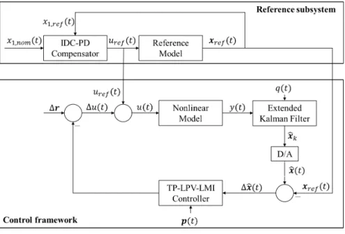
The final control structure is built up from two systems as it can be seen on Figure 1. The reference subsystem is responsible to generate the reference trajectories to be followed by the states of the original system via the control framework. It has to be pointed out that theure f(t)design method and the reference model applied in the reference subsystem can be arbitrarily selected. The main limitation is that theure f(t)realization should consider the constraints against the reference control signal described above and the applied reference model has to provide a close-to- accurate description about the connection betweenure f(t)andxre f(t).
Figure 1 Structure of the control loop.
The control framework enforces that x(t) =xre f(t),t→∞. This is the same as
∆r=x−xre f =0. Due to the fact thatx2(t)cannot be measured, it is provided by the EKF during the operation and ˆx2(t)is used for the difference generation.
4 Results of the Numerical Simulation
The realization of the control framework was done in the MATLAB framework using the forward method of Euler: dx(t0)/dt≈(x(t0+T)−x(t0))/T, where T represents the sampling time.
In accordance with the model properties we did not consider state disturbance nei- ther at the EKF design nor at simulations. Therefore, we assumed thatd≡0. How- ever, we assumed the presence of limited measurement noise with normal distribu- tion: v(t)∼N (0,502)mm3. We have taken into account this specificity during the EKF design and prepared the control framework for this action – moreover, the measurement noise only prevailed in ˆx1(t). By using the EKF, the noise appeared in theu(t)– however, in an oppressed way.
A summary of the applied circumstances can be seen in Table 2. Sincex1(t)have been considered as measurable, we assumed thatx1(t0)is available. On the other hand,x2(t0) =0 represents that there is no inhibitor in the serum before the begin- ning of the therapy. The initial state variables of the EKF were selected by con- sidering the previously mentioned facts: x1(t)is known and x2(t0) is zero. We have applied ˆx1(t0) =30100 mm3taking into account that there is a measurement noise from the beginning of the simulation. However, we have appliedx2,re f(t0) = a/b+10−3 coming from the aforementioned fact in regards to p1,min. Figure 2.
Table 1
Important indicators of the numerical simulations.
Notation Value Description
T 1 day Sampling time
Osampling [199,199]> Sampling resolution of the TP
model transformation in theΩ x(t0) [30000,0]> Initial values – original system ˆ
x(t0) [30100,0]> Initial values – EKF
xre f(t0) [30100,36.4875]> Initial values – reference system x(tf inal) [0.2949,43.9637]> Final values – original system ˆ
x(tf inal) [19.0057,43.9637]> Final values – EKF
xre f(tf inal) [0.3655,43.9547]> Final values – reference system
u(tf inal) 8.618 mg/kg/day Final value – realized control input
v(t) ∼N(0,502)mm3 Measurement noise function
presents the variation of the state variables x(t)belonging to the original system (upper part), while the middle and lower sub-figures represent the outputy(t). The x(t)varies in accordance with the control law. At the beginning, the controller rapidly intervenes into the process and decreases thex1(t)under a certain level and later it enforces the system to approach the trajectories of the reference system. The middle figure shows the outputy(t)from day 0 to day 60. It demonstrates that the magnitude of the output is too high compared to thev(t)and the measurement noise cannot be recognized on the signal. On the other hand, the lower figure presents the
output from day 60 to day 200 (end of the therapy). The effect of the noise is clearly visible in this case due to the comparable magnitudes ofy(t)andv(t).
0 20 40 60 80 100 120 140 160 180
0 1 2 3 4 104
0 50 100
0 10 20 30 40 50
0 1 2 3
104
60 80 100 120 140 160 180
0 200 400 600 800
Figure 2
Trajectories of the states and the output of the original nonlinear system.
0 20 40 60 80 100 120 140 160 180
0 2 4 104
0 50 100
0 20 40 60 80 100 120 140 160 180
0 2 4 104
0 50 100
0 20 40 60 80 100 120 140 160 180
0 1 2 3 104
0 20 40
Figure 3
Trajectories of the state variables.
The EKF approached the original model with high precision (Figure 3). The aim of the control, namely,x1(tf inal)<1 mm3has been satisfied since,x1(tf inal) =0.2949 mm3.
Figure 4. shows the discrepancies between the states of the models. The initial state error between the original model and the EKF isx(t0)−x(tˆ 0) = [−100,0]>. As we mentioned, the measurement noise only reflects in the first state – in the output – of the EKF. The error rate can be measured by applying the two norm metric on the distance: kX1−Xˆ1k2=353.4982 mm3,X1= [x1(t0),x1(t1), . . . ,x1(tf inal)]and Xˆ1= [xˆ1(t0),xˆ1(t1), . . . ,xˆ1(tf inal)]. The obtained state error is small compared to oc- curred magnitudes of the tumor volumes. The EKF behaves as an optimal estimator from the second state point’s of view since system disturbances has not been taken into consideration and sensor noise only reflects in the first state: kX2−Xˆ2k2=0 mg/kg,X2= [x2(t0),x2(t1), . . . ,x2(tf inal)]and ˆX2= [ˆx2(t0),xˆ2(t1), . . . ,xˆ2(tf inal)].
Both the original model and the EKF have approached the states of the reference model with acceptable error rate within acceptable time horizon of the therapy.
More precisely, the difference betweenx1(t), ˆx1(t)andx1,re f(t)was inside a range of 100 mm3after day 77 and continuously decreased until day 200. The deviation betweenx2(t), ˆx2(t)andx2,re f(t)was inside a range of 1 mg/kg after day 33 and continuously decreased until day 200.
Due to the small state error between the original and EKF states, the xre f(t)− ˆ
x(t)characterizes the xre f(t)−x(t)as well. Therefore, we only presented here the xre f(t)−x(tˆ ). It is clearly visible that ˆx(t) appropriately approachesxre f(t) over time. The state errors converge to zero, although thexre f(tf inal)−x(tˆ f inal) = [−18.6403,−0.0096]>due to the applied disturbance.
0 20 40 60 80 100 120 140 160 180 200
-100 -50 0 50 100
-1 -0.5 0 0.5 1
0 20 40 60 80 100 120 140 160 180 200
-1 -0.5 0 0.5 1 1.5
2 104
-80 -60 -40 -20 0 20 40
Figure 4
Deviations between the states of the models.
The comparison of the control signals can be seen in Figure 5. The upper subfigure belongs to theure f(t)and it presents that the reference control signal varies accord- ingly based on the above defined constraints. What can be pointed out is the flat region from 2 – 5 days that is the consequence of the constraint onx2,re f(t)com- ing from the already described model property: if we want to decrease the tumor volume, we need thatx2,re f(t)>a/bwhich requires thature f(t)>c·a/b.
There is the higher peak in u(t)at the beginning which decreases to zero. This immediate action is a consequence of the applied state-feedback kind control due to the initial state discrepancy betweenx2,re f(t0)and ˆx2(t0). Theure f(t)−u(t)<0.4 mg/kg/h,t>20. Small oscillations can be seen inu(t)due to the effect of the EKF.
The calculation of the totally injected inhibitor is quite easy based on Euler’s for- ward method. The IDC-PD compensator has calculated with a
120
∑
t=0
ure f(t)·T = 1567.7 mg/kg, beside, the
120 t=0
∑
u(t)·T =1600.7 mg/kg generated by the TP-LPV- LMI controller over the simulated time horizon, while
120 t=0
∑
|ure f(t)−u(t)|
=163.9821 mg/kg was the obtained difference within the time frame of the therapy.
0 20 40 60 80 100 120 140 160 180
8 10 12 14
0 20 40 60 80 100 120 140 160 180
0 20 40 60
0 20 40 60 80 100 120 140 160 180
-60 -40 -20 0
Figure 5
The reference and realized control signals.
Conclusions
The study details our latest achievements in regards to the control of tumor growth through antiangiogen therapy. Two qLPV models have been developed based on the
original nonlinear model. The Model-I has been applied during the EKF design and operation. The Model-II was used in order to design the difference based TP-LPV- LMI controller. A reference model has been also developed to describe the behavior of the first state – this was used during the reference trajectory generation.
The controller design was a complex procedure. First, we have applied TP model transformation on the Model-II. After, the control goals have been formalized by using LMIs. The procedure resulted the convex weighting functions and the con- troller vertices which built up the TP-LPV-LMI controller. We have developed a reference subsystem, as well based on IDC-PD kind compensator with the purpose of generation of the reference state variables and reference control input.
The developed control framework was tested on numerical simulations scenarios.
We have found that the system performed well and all of the control goals have been satisfied. Not just the tumor volume was decreased under a certain level, but the original nonlinear model was enforced to behave as the reference model as well.
In the future we plan to analyze the performance of the developed solutions in case of state disturbances. Moreover, we will investigate other reference signal possibil- ities as well.
Acknowledgement
This project has received funding from the European Research Council (ERC) un- der the European Union’s Horizon 2020 research and innovation programme (grant agreement No 679681). Gy. Eigner was supported by the ´UNKP-17-4-I. New Na- tional Excellence Program of the Ministry of Human Capacities.
References
[1] P. Charlton and J. Spicer. Targeted therapy in cancer. Medicine, 44(1):34–38, 2016.
[2] K. Xing and S. Lisong. Molecular targeted therapy of cancer: The progress and future prospect.Front Lab Med, 1(2):69–75, 2017.
[3] N.S. Vasudev and A.R. Reynolds. Anti-angiogenic therapy for cancer: cur- rent progress, unresolved questions and future directions. Angiogenesis, 17(3):471–494, 2014.
[4] B. Al-Husein, M. Abdalla, M. Trepte, D.L. DeRemer, and P.R. Somanat. Anti- angiogenic therapy for cancer: An update. Pharmacotherapy, 32(12):1095–
1111, 2012.
[5] Y. Kubota. Tumor angiogenesis and antiangiogenic therapy.Keio J Med, 61:47 – 56, 2012.
[6] J. S´ajevics´e S´api. Controller-managed automated therapy and tumor growth model identification in the case of antiangiogenic therapy for most effective, individualized treatment. PhD thesis, Applied Informatics and Applied Math- emathics Doctoral School, ´Obuda University, Budapest, Hungary, 2015.
[7] A.M.E. Abdalla, L. Xiao, M. Wajid Ullah, M. Yu, C. Ouyang, and G. Yang.
Current challenges of cancer anti-angiogenic therapy and the promise of nan- otherapeutics. Theranostics, 8(2):533–548, 2018.
[8] J.K. Tar, J. Bit´o, L. N´adai, and JA Tenreiro Machado. Robust fixed point trans- formations in adaptive control using local basin of attraction. Acta Polytech Hung, 6(1):21–37, 2009.
[9] A. Dineva, J.K. Tar, A. V´arkonyi-K´oczy, and V. Piuri. Adaptive controller us- ing fixed point transformation for regulating propofol administration through wavelet-based anesthetic value. In2016 IEEE International Symposium on Medical Measurements and Applications (MeMeA), pages 1–6. IEEE, 2016.
[10] L. Kov´acs. A robust fixed point transformation-based approach for type 1 diabetes control.Nonlin Dyn, 89(4):2481–2493, 2017.
[11] D. Copot, R. De Keyser, J. Juchem, and C.M. Ionescu. Fractional order impedance model to estimate glucose concentration: in vitro analysis. Acta Polytech Hung, 14(1):207–220, 2017.
[12] C. Ionescu, R. De Keyser, J. Sabatier, A. Oustaloup, and F. Levron. Low fre- quency constant-phase behavior in the respiratory impedance. Biomed Signal Proces, 6(2):197–208, 2011.
[13] C. Ionescu, A. Lopes, D. Copot, J.A.T. Machado, and J.H.T. Bates. The role of fractional calculus in modeling biological phenomena: A review. Commun Nonlinear Sci, 51:141–159, 2017.
[14] F.S. Lobato, V.S. Machado, and V. Steffen. Determination of an optimal con- trol strategy for drug administration in tumor treatment using multi-objective optimization differential evolution. Comp Meth Prog Biomed, 131:51–61, 2016.
[15] D. Drexler, J. S´api, and L. Kov´acs. Potential Benefits of Discrete-Time Controller-based Treatments over Protocol-based Cancer Therapies. Acta Polytech Hung, 14(1):11–23, 2017.
[16] J. Klamka, H. Maurer, and A. Swierniak. Local controllability and optimal control for amodel of combined anticancer therapy with control delays.Math Biosci Eng, 14(1):195–216, 2017.
[17] D.A. Drexler, J. S´api, and L. Kov´acs. Modeling of tumor growth incorporating the effects of necrosis and the effect of bevacizumab.Complexity, 2017:1–10, 2017.
[18] D.A. Drexler, J. S´api, and L. Kov´acs. Positive control of a minimal model of tumor growth with bevacizumab treatment. In Proceedings of the 12th IEEE Conference on Industrial Electronics and Applications, pages 2081–
2084, 2017.
[19] L. Kov´acs. Linear parameter varying (LPV) based robust control of type-I diabetes driven for real patient data. Knowl-Based Syst, 122:199–213, 2017.
[20] P. Baranyi, Y. Yam, and P. Varlaki. Tensor Product Model Transformation in Polytopic Model-Based Control. Series: Automation and Control Engineering.
CRC Press, Boca Raton, USA, 1st edition, 2013.
[21] M.S. Grewal and A.P. Andrews.Kalman Filtering: Theory and Practice Using MATLAB. John Wiley and Sons, Chichester, UK, 3rd edition, 2008.
[22] D. Drexler, J. S´api, and L. Kov´acs. A minimal model of tumor growth with angiogenic inhibition using bevacizumab. InSAMI 2017 - IEEE 15th Inter- national Symposium on Applied Machine Intelligence and Informatics, pages 185 – 190. IEEE.
[23] D.A. Drexler, J. S´api, and L. Kov´acs. Positive nonlinear control of tumor growth using angiogenic inhibition.IFAC-PapersOnLine, 50(1):15068–15073, 2017.
[24] Y. Akatsu, Y. Yoshimatsu, T. Tomizawa, K. Takahashi, A. Katsura, K. Miya- zono, and T. Watabe. Dual targeting of vascular endothelial growth factor and bone morphogenetic protein-9/10 impairs tumor growth through inhibition of angiogenesis.Cancer Science, 108(1):151–155, 2017.
[25] J. S´api, L. Kov´acs, D.A. Drexler, P. Kocsis, D. Ga´ari, and Z. S´api. Tumor volume estimation and quasi-continuous administration for most effective be- vacizumab therapy.PLoS ONE, 10(11), 2015.
[26] O. Sename, P. G´asp´ar, and J. Bokor. Robust control and linear parameter varying approaches, application to vehicle dynamics. volume 437 ofLecture Notes in Control and Information Sciences. Springer-Verlag, Berlin, 2013.
[27] A.P. White, G. Zhu, and J. Choi. Linear Parameter Varying Control for Engi- neering Applicaitons. Springer, London, 1st edition, 2013.
[28] C. Briat. Linear parameter-varying and time-delay systems. Analysis, Obser- vation, Filtering & Control, 3, 2014.
[29] Gy. Eigner. Closed-Loop Control of Physiological Systems. PhD thesis, Ap- plied Informatics and Applied Mathemathics Doctoral School, ´Obuda Univer- sity, Budapest, Hungary, 2017.
[30] P. Baranyi. TP-model Transformation-based-control Design Frameworks.
Springer, 2016.
[31] P. Baranyi. Extension of the Multi-TP Model Transformation to Functions with Different Numbers of Variables. Complexity, 2018, 2018.
[32] L-E. Hedrea, C-A. Bojan-Dragos, R-E. Precup, R-C. Roman, E.M. Petriu, and C. Hedrea. Tensor product-based model transformation for position control of magnetic levitation systems. In2017 IEEE 26th International Symposium on Industrial Electronics (ISIE), pages 1141–1146. IEEE, 2017.
[33] L-E. Hedrea, C-A. Bojan-Dragos, R-E. Precup, and T-A. Teban. Tensor product-based model transformation for level control of vertical three tank sys-
tems. In2017 IEEE 21st International Conference on Intelligent Engineering Systems (INES), pages 000113–000118. IEEE, 2017.
[34] J.D. Bronzino and D.R. Peterson, editors. The Biomedical Engineering Hand- book. CRC Press, Boca Raton, USA, 4th edition, 2016.
[35] J. Kuti, P. Galambos, and P. Baranyi. Minimal volume simplex (MVS) convex hull generation and manipulation methodology for TP model transformation.
Asian J Control, 19(1):289–301, 2017.
[36] J. Kuti, P. Galambos, and P. Baranyi. Control analysis and synthesis through polytopic tensor product model: a general concept. IFAC-PapersOnLine, 50(1):6558–6563, 2017.
[37] P. Galambos and P. Baranyi. TP model transformation: A systematic mod- elling framework to handle internal time delays in control systems. Asian J Control, 17(2):1 – 11, 2015.
[38] P. Baranyi. The generalized TP model transformation for T–S fuzzy model manipulation and generalized stability verification. IEEE T Fuzzy Syst, 22(4):934–948, 2014.
[39] Sz. Nagy, Z. Petres, P. Baranyi, and H. Hashimoto. Computational relaxed TP model transformation: restricting the computation to subspaces of the dynamic model.Asian J Control, 11(5):461–475, 2009.
[40] J. Cui, K. Zhang, and T. Ma. An efficient algorithm for the tensor product model transformation.Int J Control Autom, 14(5):1205–1212, 2016.
[41] A. Szollosi and P. Baranyi. Influence of the Tensor Product model represen- tation of qLPV models on the feasibility of Linear Matrix Inequality. Asian J Control, 18(4):1328–1342, 2016.
[42] A. Szollosi and P. Baranyi. Improved control performance of the 3-DoF aeroe- lastic wing section: a TP model based 2D parametric control performance op- timization. Asian J Control, 19(2):450–466, 2017.
[43] A. Szollosi and P. Baranyi. Influence of the Tensor Product Model Represen- tation of qLPV Models on the Feasibility of Linear Matrix Inequality Based Stability Analysis. Asian J Control, 20(1):531–547, 2018.
[44] P. V´arkonyi, D. Tikk, P. Korondi, and P. Baranyi. A new algorithm for RNO- INO type tensor product model representation. In2005 IEEE International Conference on Intelligent Engineering Systems, INES, volume 5, pages 263–
266, 2005.
[45] X. Liu, Y. Yu, Z. Li, Herbert H.C. Iu, and T. Fernando. An Efficient Algorithm for Optimally Reshaping the TP Model Transformation. IEEE T Circuits-II, 64(10):1187–1191, 2017.
[46] X. Liu, X. Xin, Z. Li, and Z. Chen. Near Optimal Control Based on the Tensor- Product Technique.IEEE T Circuits-II, 64(5):560–564, 2017.
[47] X. Liu, Y. Yu, Z. Li, and H. Iu. Polytopic H∞filter design and relaxation for nonlinear systems via tensor product technique.Signal Process, 127:191–205, 2016.
[48] X. Liu, Y. Yu, H. Li, Z.and Iu, and Ty. Fernando. A novel constant gain Kalman filter design for nonlinear systems.Signal Process, 135:158–167, 2017.
[49] P.S. Saikrishna, R. Pasumarthy, and N.P. Bhatt. Identification and multivari- able gain-scheduling control for cloud computing systems. IEEE T Cont Syst T, 25(3):792–807, 2017.
[50] G. Zhao, D. Wang, and Z. Song. A novel tensor product model transformation- based adaptive variable universe of discourse controller. J Frankl Inst, 353(17):4471–4499, 2016.
[51] W. Qin, B. He, Q. Qin, and G. Liu. Robust active controller of hypersonic vehicles in the presence of actuator constraints and input delays. In2016 35th Chinese Control Conference (CCC), pages 10718–10723. IEEE, 2016.
[52] Q. Weiwei, H. Bing, L. Gang, and Z. Pengtao. Robust model predictive track- ing control of hypersonic vehicles in the presence of actuator constraints and input delays. J Frankl Inst, 353(17):4351–4367, 2016.
[53] T. Wang and B. Liu. Different polytopic decomposition for visual servoing system with LMI-based Predictive Control. In 2016 35th Chinese Control Conference (CCC), pages 10320–10324. IEEE, 2016.
[54] T. Wang and W. Zhang. The visual-based robust model predictive control for two-DOF video tracking system. In2016 Chinese Control and Decision Conference (CCDC), pages 3743–3747. IEEE, 2016.
[55] T. Jiang and D. Lin. Tensor Product Model-Based Gain Scheduling of a Mis- sile Autopilot.T Jpn Soc Aeronaut S, 59(3):142–149, 2016.
[56] S. Campos, V. Costa, L. Tˆorres, and R. Palhares. Revisiting the TP model transformation: Interpolation and rule reduction. Asian J Control, 17(2):392–
401, 2015.
[57] S. Kuntanapreeda. Tensor Product Model Transformation Based Control and Synchronization of a Class of Fractional-Order Chaotic Systems.Asian J Con- trol, 17(2):371–380, 2015.
[58] R-E. Precup, E.M. Petriu, M-B. R˘adac, S. Preitl, L-O. Fedorovici, and C- A. Dragos¸. Cascade Control System-Based Cost Effective Combination of Tensor Product Model Transformation and Fuzzy Control. Asian J Control, 17(2):381–391, 2015.
[59] P. Korondi. Tensor product model transformation-based sliding surface design.
Acta Polytech Hung, 3(4):23–35, 2006.
[60] Gy. Eigner, I. B¨ojthe, P. Pausits, and L. Kov´acs. Investigation of the tp model- ing possibilities of the hovorka t1dm model. In2017 IEEE 15th International
Symposium on Applied Machine Intelligence and Informatics (SAMI), pages 259–264. IEEE, 2017.
[61] Gy. Eigner, P. Pausits, and L. Kov´acs. Control of t1dm via tensor product- based framework. In2016 IEEE 17th International Symposium on Computa- tional Intelligence and Informatics (CINTI), pages 55–60. IEEE, 2016.
[62] Gy. Eigner, I. Rudas, A. Szak´al, and L. Kov´acs. Tensor product based mod- eling of tumor growth. In2017 IEEE International Conference on Systems, Man, and Cybernetics (SMC), pages 900–905. IEEE, 2017.
[63] L. Kov´acs and Gy. Eigner. Usability of the tensor product based modeling in the modeling of diabetes mellitus.Manuscript in preparation, 2016.
[64] Gy. Eigner, I. Rudas, and L. Kov´acs. Investigation of the tp-based modeling possibility of a nonlinear icu diabetes model. In2016 IEEE International Con- ference on Systems, Man, and Cybernetics (SMC), pages 3405–3410. IEEE, 2016.
[65] L Kov´acs and Gy. Eigner. Convex polytopic modeling of diabetes mellitus:
A tensor product based approach. In2016 IEEE International Conference on Systems, Man, and Cybernetics (SMC), pages 003393–003398. IEEE, 2016.
[66] J. Klespitz, I. Rudas, and L. Kov´acs. LMI-based feedback regulator design via TP transformation for fluid volume control in blood purification therapies.
In 2015 IEEE International Conference on Systems, Man, and Cybernetics (SMC), pages 2615–2619. IEEE, 2015.
[67] J. Kuti, P. Galambos, and ´A. Mikl´os. Output Feedback Control of a Dual- Excenter Vibration Actuator via qLPV Model and TP Model Transformation.
Asian J Control, 17(2):432–442, 2015.
[68] J. Pan and L. Lu. TP Model Transformation Via Sequentially Truncated Higher-Order Singular Value Decomposition.Asian J Control, 17(2):467–475, 2015.
[69] J. Matuˇsko, ˇS. Ileˇs, F. Koloni´c, and V. Leˇsi´c. Control of 3d tower crane based on tensor product model transformation with neural friction compensation.
Asian J Control, 17(2):443–458, 2015.
[70] G. Zhao, H. Li, and Z. Song. Tensor product model transformation based decoupled terminal sliding mode control. Int J Syst Sci, 47(8):1791–1803, 2016.
[71] S. Chumalee and J. Whidborne. Gain-Scheduled H∞Control for Tensor Prod- uct Type Polytopic Plants.Asian J Control, 17(2):417–431, 2015.
[72] R-E. Precup, C-A. Dragos, S. Preitl, M-B. Radac, and E-M. Petriu. Novel tensor product models for automatic transmission system control. IEEE Syst J, 6(3):488–498, 2012.
[73] R-E. Precup, M-Cs. Sabau, and E.M. Petriu. Nature-inspired optimal tuning of input membership functions of takagi-sugeno-kang fuzzy models for anti-lock braking systems. Appl Soft Comput, 27:575–589, 2015.
[74] R-E. Precup, R-C. David, and E.M. Petriu. Grey wolf optimizer algorithm- based tuning of fuzzy control systems with reduced parametric sensitivity.
IEEE T Ind Electron, 64(1):527–534, 2017.
[75] K. Tanaka and H.O. Wang. Fuzzy Control Systems Design and Analysis: A Linear Matrix Inequality Approach. John Wiley and Sons, Chichester, UK, 1st edition, 2001.
[76] S. Boyd, L. El Ghaoui, E. Feron, and V. Balakrishnan. Linear Matrix Inequal- ities in System and Control Theory, volume 15 ofStudies in Applied Mathe- matics. SIAM, Philadelphia, PA, June 1994.
[77] H. Musoff and P. Zarchan. Fundamentals of Kalman Filtering: A Practical Approach. American Institute of Aeronautics and Astronautics, 3rd edition, 2009.
[78] J. Hartikainen, A. Solin, and S. S¨arkk¨a.Optimal Filtering with Kalman Filters and Smoothers a Manual for the Matlab toolbox EKF/UKF. Aalto University, v1.3 edition, 2011.
[79] Y. Tagawa, J.Y. Tu, and D.P. Stoten. Inverse dynamics compensation via simu- lation of feedback control systems.Proceedings of the institution of mechani- cal engineers, Part I: Journal of systems and control engineering, 225(1):137–
153, 2011.
[80] B. Siciliano, L. Sciavicco, L. Villani, and G. Oriolo. Robotics–Modelling, Planning and Control. Advanced Textbooks in Control and Signal Processing Series. Springer-Verlag, 2009.
Notations and Abbreviations
Table 2 General Phrases.
Abbreviation Meaning
LTI Linear Time Invariant LTV Linear Time Variant LPV Linear Parameter Varying
qLPV quasi LPV
TP model Tensor Product model LMI Linear Matrix Inequality MVS Minimal Volume Simplex SVD Singular Value Decomposition HOSVD Higher-Order SVD
EKF Extended Kalman Filter
Table 3 Mathematical terms.
Notation Meaning a,b, ... scalars a,b, . . . vector A,B, . . . matrices
ai,bi, . . . ith row vector ofA,B, . . .matrices
ai,j,bi,j, . . . jth elements of theai,bi, . . .row vectors
A,B, . . . tensors
S N
n=1Wn multiple tensor products,
e.g.S×1W1. . .×NWN
R,C, . . . mathematical sets
![Figure 4. shows the discrepancies between the states of the models. The initial state error between the original model and the EKF is x(t 0 ) − x(tˆ 0 ) = [−100,0] >](https://thumb-eu.123doks.com/thumbv2/9dokorg/1237617.95470/14.748.153.603.610.924/figure-shows-discrepancies-states-models-initial-state-original.webp)
