Optimal PID Based Computed Torque Control of Tumor Growth Models ⋆

Optimal PID Based Computed Torque Control of Tumor Growth Models ⋆

Bence G. Czak´o, Johanna S´api,Levente Kov´acs

Physiological Controls Research Center, Research, Innovation, and Service Center, ´Obuda University Budapest, Hungary (email:

czako.bence@stud.uni-obuda.hu,{kovacs.levente, sapi.johanna}@nik.uni-obuda.hu)

Abstract:In the past few decades cancer research has delivered several new treatment options, of which can be highly expensive thus reducing its applicability in medical practice. However, advances in control engineering can tackle this issue by the use of an appropriate optimal controller. In this paper a Computed Torque Control (CTC) based PID controller was designed for the Hahnfeldt tumor growth model which can provide an optimal administration protocol for every individual patient. The paper contains the system model in conjunction with the detailed design steps of the controller. The control strategy was tested by numerical simulations which can be found at the end of the paper together with the conclusions.

Keywords:Computed Torque Control, PID Control, LQR tuning, Tumor Growth Model, Hahnfeldt Model

1. INTRODUCTION

Cancerous diseases are one of the most serious illnesses of modern society which cause high mortality rates. Ac- cording to Malvezzi et al. (2017), approximately 1 373 500 people died in 2017 due to cancer which is a 3% increase compared to 2012. These high numbers can be attributed to inefficient treatment strategies such as chemotherapy or radiotherapy which often has adverse impact on the health of the patient.

Researchers have developed a number of new method- ologies from which targeted molecular therapies (TMT) offers promising results (Charlton and Spicer (2016)). In particular anti-angiogenic treatment has been a significant advancement which targets special tumor growth mecha- nisms. In theory the side effects are mild compared to con- ventional protocols which renders the method attractive to medical professionals (Harris (2003)).

Besides its promising features, anti-angiogenic treatment has numerous disadvantages. Based on Jayson et al.

(2016), the drug has no effect on particular cancer illnesses, prostate or pancreatic cancer for example. However, it is also worth noting that nowadays the protocol is vastly applied as a combined treatment in practice (Ilic et al.

(2016)). From biological perspective future research should scrutinise predictive biomarkers, however from an engi- neering standpoint a different problem will be discussed in this paper that is the treatment often infers high medical expenses which should be addressed in order to be applied widely.

⋆ This project has received funding from the European Research Council (ERC) under the European Unions Horizon 2020 research and innovation programme (grant agreement No 679681). B.G.

Czak was supported by the UNKP-17-2/I. New National Excellence Program of the Ministry of Human Capacities.

In the recent years biomedical control has become a flour- ishing discipline in engineering. Mathematical models are employed on physiological processes which can lead to effective individualized treatment solutions, Ionescu et al.

(2011) and Ionescu et al. (2017) for example, and curing cancer is not an exception as well. From a control engi- neering perspective the tumor regulation problem can be solved using an optimal controller which aims to decrease the size of the tumor in the shortest manner while mini- mizing the magnitude of input signal i.e. the concentration of the medication. In order to design such a controller an appropriate model should be used which describes the tumor growth under anti-angiogenic inhibition. An impor- tant growth model is the Hahnfeldt model introduced by Hanhfeldt et al. (1999). While the model seems simple at first glance, it has severe nonlinearities which should be handled with care.

Several linear control methods were proposed by various authors in order to control the volume of the tumor. In S´api et al. (2015) the authors investigated several linear strategies including pole placement and LQR design, while Kovacs et al. (2013) analyzed modern robust control pos- sibilities. Although these controllers provided significantly better results compared to existing medical protocols, they are not exploiting the nonlinearities which could improve the overall performance of the treatment. Nonlinear tech- niques were investigated in Czak´o et al. (2017) or Drexler et al. (2017a) such as nonlinear model predictive control (NMPC), robust fixed point transformation (RFPT) based control and exact linearization in order to decrease the total inhibitor concentration while improving robustness of the controlled system.

In this paper, a different nonlinear strategy is proposed which is not computationally expensive and shares the important traits of the other controllers. Section 2 gives

a brief description on the considered tumor growth model, while Section 3 and 4 presents the control concept in the context of RFPT control design. In Section 5 the proposed algorithm is validated by numerical simulations followed by conclusions and further research possibilities in Section 6.

2. THE SIMPLIFIED TUMOR GROWTH MODEL In order to create a stabilizing controller, a proper tumor growth model under anti-angiogenic inhibition is indis- pensable. The basic model is (still) considered the work of Hanhfeldt et al. (1999) although some phenomena is not covered by it.

As a result, several models were proposed by various authors including Drexler et al. (2017b) and Csercsik et al. (2017) in order to include recent pathophysiological advancements in the process model, however in this paper we are still considering the original Hahnfeldt model as the main idea is to demonstrate the applicability of the introduced control methodology in comparison with other approaches used on the same model.

Based on Sapi et al. (2013) a simplification of the original Hahnfeldt model can be carried out which has the follow- ing form:

˙

x₁=−λx₁ln (x1

x₂ )

˙

x₂=bx₁−dx^2/3₁ x₂−ex₂g(t) y=x1

(1)

where x1 denotes the tumor volume (mm³) representing the output of the model as well, x2 is the volume of the tumor vasculature (mm³), λ is the growth parameter of the tumor (1/day), b is the angiogenic factor (1/day), d describes the cellular blocking mechanisms of the vascula- ture (1/day·mm²),e is the inhibition of the vasculature by the drug (kg/day·mg), andg(t) is the concentration of the administered inhibitor (mg/kg) considered the input of the model.

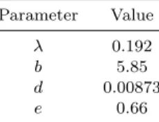
One should be aware, that the model has a singularity at x1 = 0, x2 = 0 which implies that the tumor can not be eradicated. However, the main goal of the research is to tame the cancer by decreasing the size of the tumor to a point where it does not pose any threat to the patient health. Simulation parameters were chosen according to S´api et al. (2015) which are presented in Table 1.

Table 1. Simulation parameters

Parameter Value

λ 0.192

b 5.85

d 0.00873

e 0.66

With these parameters and constant zero inhibitor ad- ministration, the final value of the state variables are x1 = x2 = 1.734·10⁴ mm³; hence, these values will be used as initial conditions.

Therefore, the main goal of the control algorithm is to govern the system from an arbitrary initial state (which is less or equal than the maximal value without inhibition) to a safe steady state tumor volume, preferably smaller than 10mm³.

3. THE FEEDBACK LINEARIZATION APPROACH In order to steer the states to the desired regime, an appro- priate controller should be designed. Besides, the controller should minimize the control effort so that expenses are smaller compared to current medical protocols. In this paper, a feedback linearization-based controller is utilized, with and LQR-based tuning rule. Suppose that the first equation of 1 can be expressed as:

¨

x1=−x˙1λln (x1

x2

)

−λx˙1+λx1x˙2

x2

(2) If ˙x2 is substituted into (2) one can obtain the following form:

¨

x1=−x˙1λln (x1

x2

)

−λx˙1+bλx²₁ x2−λdx

5 3

1 −eλx1g(t) (3) By choosing a suitable input signal, ¨x1 can be linearized.

Therefore,g(t) can be determined as:

g(t) =−x˙1λln(x₁ x₂

)+λx˙1−bλx²₁ x₂ +λdx

5 3

1 +u eλx1

(4) whereuis an auxiliary control input. Note that now ¨x₁=u which is linear. Equation (4) can be further simplified to:

g(t) =−λ( ˙x1(ln(x1

x2

)+ 1)−bx²₁ x2 +dx

5 3

1) +u

eλx₁ (5)

In order to govern the volume of the tumor one should consider defining the error between the desired and actual states, namely:

e=x₁−x^d₁ (6) wherex^d₁is the desired tumor volume which is determined by the control objective. Differentiating the error two times leads to:

˙

e= ˙x₁−x˙^d₁

¨

e= ¨x1−x¨^d₁ (7) One can see that the second equation contains the linear term ¨x1 which produces:

¨

e= ¨x₁−x¨^d₁=u−x¨^d₁= ˆu (8) If one defines the error vector ase= [e e]˙^T the following linear system can be obtained:

[

˙ e

¨ e ]

= [

0 1 0 0

] [ e

˙ e ]

+ [

0 1 ]

ˆ

u (9)

which is equivalent to:

˙

e=Ae+Buˆ (10) Assume that a static feedback is defined in the form of ˆ

u = −Ke, where K is constructed so that it minimizes the functional:

J =

∫ _∞

0

e^TQe+µˆu²dt (11) In (11), µ > 1 penalize the control effort (note that in general the second term should be ˆu^TRu, butˆ R is now just a constant term), andQis the error weighting matrix as follows:

Q= [ξ1 0

0 ξ₂ ]

(12) whereξ₁andξ₂ are responsible for the tracking precision.

Upon possessing A, B, Q, R, one can calculate the gain matrixKanalytically byK=R⁻¹B^TP, wherePis the so- lution of the Ricatti equationA^TP+P A−P BR⁻¹B^TP+ Q = 0. In this case, the gain matrix K is just a vector, preciselyK= [k1 k2]. Substituting ˆu=−Keinto (8) one can calculateuas follows:

u= ¨x1+ ˆu= ¨x1−k2e˙−k1e (13) The last step is to obtainx2 in (5). In this case,x2can be calculated from the desired tumor volume as follows:

x₂=x^d₁ exp⁻¹ ( x˙^d₁

−λx^d₁ )

(14) Using these equations, a stable controller can be utilized.

In each control cycle the error between the desired and actual tumor volume is computed altogether with its first derivative so that e can be obtained by (6) and (7). In the next step, the value of uis determined by (13) based on preliminary calculation of the gain vectorK. By using (14), the appropriate value ofx₂can be carried out which then substituted into (5) in conjunction withuresults in the control signal g(t) that is applied to the plant.

In the next section, a slightly robust version of the con- troller is presented which uses the RFPT based control technique. In theory this augmentation improves the per- formance of the controller; however, there is no tuning technique of the RFPT method which results in an optimal control sequence, therefore it can not be utilized by itself.

4. AUGMENTED ROBUST FIXED POINT TRANSFORMATION BASED CONTROLLER The idea of the RFPT method originates from Tar et al.

(2009) in which the underlying idea is to construct an inverse model of the system that is connected to a sliding

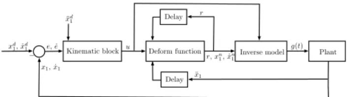
Deform function

Kinematic block Inverse model Plant

Delay

Delay x^d₁, ˙x^d₁

¨ x^d₁

e, ˙e u

− r,xⁿ1, ˙xⁿ1

r

g(t)

x1, ˙x1

¨ x1

Fig. 1. A schematic depiction of the control loop.

mode (SM) controller, called the kinematic block. This SM controller is then connected to a deformation block that can properly manipulate the corresponding state variables which then applied on the inverse model results in a proper control input. A more detailed explanation of the method can be found in Tar et al. (2012).

The original idea was applied in Czak´o et al. (2017) never- theless it does not impose any penalty on the input signal.

In this paper a slightly modified version of the RFPT controller was designed which only uses the deformation block altogether with the feedback linearization approach.

This entails that the kinematic block is replaced by (13), where the gains are determined by the LQR tuning and not the original operator which is:

(d

dt+ Λ)ⁿ⁺¹eint= 0 (15) where eint is the integral of the error, Λ is a controller parameter andnis the order of the control task. Note that in this case, the controller does not require the integral of the error term. Using the fact that ¨x₁ =u, based on the inverse model (5), a deformation is applied to the system.

In this SISO case, the deform function can be defined as:

G(r|u)^def= (r+K)[1 +Btanh(A[f(r)−u])]−K G(u_∗|u) =u_∗ iff(u_∗) =u

G(−K|u) =−K ifr=−K

(16) which then is iterated as rn+1 = G(rn|u). In (16), A, B andK are the control parameters,f(r) is the response of the system for the deformed inputr,u_∗is the fixed point of the equation, and the role ofris to maintain the iteration.

In each control cycle, the value of r is used to compute x2 by (14) that is substituted into (5) in conjunction with u. The missing x₁ and ˙x₁ can be computed from r by integrating it two times. Note that ifr=u_∗ the input of the deform block equals with the output, so thatu_∗= ¨x₁, which justifies the integration. It is also worth mentioning that the iteration entails two time delays which coincide with the step size of the simulation. On Fig. 1 a simple sketch of the control loop is presented in order to facilitate the understanding of the RFPT algorithm.

For the desired trajectory, multiple prescriptions were con- sidered. First, a heuristic tanh() function based trajectory is proposed based on Czak´o et al. (2017), which has the following general form:

x^d₁(t) = (−tanh(ct) + 1)(x^s₁−x^f₁) +x^f₁ (17)

wherec >0 is a scaling constant,x^s₁ is the initial value of the tumor volume and 0< x^f₁ ≤10 denotes its final value.

Differentiating the expression above twice leads to:

˙

x^d₁(t) =c(x^s₁−x^f₁)sech²(ct)

¨

x^d₁(t) =−2c²(x^f₁−x^s₁)sech²(ct)tanh(ct) (18) The problem with this prescription is that at t = 0 the first derivative is not zero which may cause high initial dosage levels. A remedy to this issue could be provided by an exponential function based trajectory which is defined according to Rymansaib et al. (2013) as:

x^d₁(t) = exp((−ct)³)(x^s₁−x^f₁) +x^f₁ (19) and their first and second derivatives are:

˙

x^d₁(t) = 3c³exp(−c³t³)(x^f₁−x^s₁)t²

¨

x^d₁(t) =−3c³exp(−c³t³)(x^f₁−x^s₁)t(−2 + 3c³t³) (20) Observing the above expressions one can easily deduce that att= 0 the derivatives are both zero which solves the problem. A third set point prescription was also defined as a constantx^d₁(t) =x^f₁ with zero derivatives.

5. NUMERICAL SIMULATION

Several simulations were conducted in order to measure the qualitative behaviour of the proposed control algo- rithms. The model parameters were indicated in Table 1. before, with the corresponding initial values of the tumor and its vasculature of x1=x2 = 1.734·10⁴ mm³. Therefore, the value x^s₁ = 1.734·10⁴ mm³ was assigned to the prescriptions in conjunction withx^f₁ = 1mm³. The scaling constant of the tanh() and exponential case were bothc= 0.1. By these choices, the tumor volume reduces to a safe level in 30 days both cases. The initial controller parameters can be seen in Table 2 which was determined on the basis of numerical simulations. In order to tune the controller, the RFPT part must be adjusted first with the original operator (15) in conjunction with Λ = 1 so that the tracking error is minimal. After that the LQR parameters can be set so that they fulfill the treatment cri- teria. The simulation time was 100days, and a continuous therapy was assumed. One should note, that continuous treatment is not likely to be possible because a proper feedback is not available, however it can be employed to investigate the basic properties of the controllers.

Table 2. Initial controller parameters for the tanh() tracking

Parameter Value

ξ1 10⁷

ξ2 1

µ 10

K 7·10¹⁰

A 10⁻¹¹

B −1

The simple LQR controller was scrutinised first. Simu- lations showed that it could track the tanh() signal ef-

ficiently. On Fig. 3. one can see, that the error for the initial control parameters was high at the beginning, but reduces to zero in finite time. If one increase the value of ξ1, more accurate tracking can be obtained. On Fig. 4. the administration protocol can be viewed. It is notable that because the trajectory prescription has non zero derivative at time t = 0, there is a jump at the beginning of the administration. It should also be clear, that negative input is not possible (one can not remove inhibitor from the pa- tient) which means that a saturation had to be employed to the system that limits the input signal magnitude between 0mg/kgand 30mg/kg. The purpose of the upper bound is to avoid high dosage profiles which could jeopardize the health of the patient. The reduction of both tumor and vasculature volume can be seen on Fig. 2.

0 10 20 30 40 50 60 70 80 90 100

Time (days) 0

0.5 1 1.5 2

Volumes (mm3) 10⁴

Vasculature volume Tumor volume

Fig. 2. Reduction of the volumes by using tanh() prescrip- tion.

0 10 20 30 40 50 60 70 80 90 100

Time (days) 0

50 100 150

Tumor volume error (mm3) ^Error

Fig. 3. Error of the tumor volume by using tanh() pre- scription.

0 10 20 30 40 50 60 70 80 90 100

Time (days) -40

-30 -20 -10 0 10 20 30

Concentration (mg/kg)

Inhibitor concentration

Fig. 4. Inhibitor profile by using tanh() prescription.

The next simulations targeted the constant reference case.

Here, the desired volume wasx^d₁(t) =x^f₁ = 1mm³and the derivatives were both zero. Multiple simulations showed, that the best results can be obtained if one setsξ1=ξ2= 1 altogether with µ ∈ [100; 1000]. By varying µ different

settling times and inhibitor profiles can be achieved, which entails that larger µ values leads to slower settling time and lower dosage profile. On Fig. 5. one can view the reduction of the tumor and vasculature volumes. It has similar characteristic as the tanh() case, but it reaches a safe level considerably faster. The corresponding inhibitor profile can be seen on Fig. 6. It should be noted that under a 100 days period the volume only reached 1.79 mm³, which is not identical to the desired prescription. However, one should consider that under 10mm³tumor volume the treatment is successful, and by increasing the simulation time the error term vanishes.

In the case of the exponential trajectory, the results were unsatisfying. While the controller could track the trajectory with minimal error, the inhibitor dosage profile was unacceptable due to high concentration levels, hence this type of trajectory is omitted.

Simulations showed, that the augmented RFPT controller has not proven to be useful with parameters included in Table 2. The tracking error grew significantly, while the inhibitor profile became inconsistent which can be seen on Fig. 7. It was not possible to remove the negative values with a saturation as well, because it destabilized the system. On Fig. 8. one can see that compared to the tanh() case, the error differs considerably and the corresponding reduction is shown on Fig. 9. The poor performance of the controller can be attributed to the structure of the kinematic block. Compared to the original prescription (15), the LQR based PID controller has slower convergence rate which results in higher tracking error and initial oscillations in the control signal. Unfortunately this behaviour can not be alleviated by varying the control parameters of the LQR or RFPT functions which means that the PD type structure of the kinematic block is inadequate for the RFPT controller.

0 10 20 30 40 50 60 70 80 90 100

Time (days) 0

5000 10000 15000

Volumes (mm3)

Vasculature volume Tumor volume

Fig. 5. Reduction of the volumes by using constant set point tracking.

Compared to other controllers, the augmented RFPT con- troller obviously did not perform well, however the PID controller in the constant reference case has many promis- ing features. By varying parameter µ different control strategies can be created which may have a longer time span but uses lower dosages. This is also true for the tanh() case, where by changing the value of parameter c in the trajectory prescription leads to the same effect as before.

In addition the huge similarity between the constant and tanh() inhibitor profiles implies some connection between both methods, which means that by using the tanh()

prescription, a fully customized treatment plan can be constructed.

0 10 20 30 40 50 60 70 80 90 100

Time (days) 10

15 20 25 30

Concentration (mg/kg)

Inhibitor concentration

Fig. 6. Inhibitor profile by using constant set point track- ing.

0 10 20 30 40 50 60 70 80 90 100

Time (days) -20

-10 0 10 20 30 40 50

Concentration (mg/kg)

Inhibitor concentration

Fig. 7. Inhibitor profile in the case of the augmented RFPT controller.

0 10 20 30 40 50 60 70 80 90 100

Time (days) 0

100 200 300 400 500

Tumor volume error (mm3)

Error

Fig. 8. Error of the tumor volume in the case of the augmented RFPT controller.

0 10 20 30 40 50 60 70 80 90 100

Time (days) 0

0.5 1 1.5 2

Volumes (mm3) 10⁴

Vasculature volume Tumor volume

Fig. 9. Reduction of the volumes in the case of the augmented RFPT controller.

6. CONCLUSION

In this paper a control engineering based approach was presented in order to lower the medical expenses of the antiangiogenic TMT treatment. A feedback linearization- based controller was designed, which based on the Hahn- feldt model could track various tumor volume prescriptions including set point tracking as well. A modified approach was presented as well which in theory could improve the performance of the PID controller. Simulations showed however that this augmented RFPT controller was not operated as expected. In order to be applicable, several other features of the PID controller has to be investigated.

Robustness for example rises many questions regard to model parameters and measurement disturbances. Since system parameters are highly unlikely to be an accurate representation of the reality, the parameter robustness of the system is essential in order to be employed in every day practice. Discrete time control also has to be sim- ulated due to the lack of continuous measurement, and has to compensate for the time intervals between inhibitor dosages. These effects altogether can cause the system to be unstable which leads to ineffective treatment.

REFERENCES

Charlton, P. and Spicer, J. (2016). Targeted therapy in cancer. Medicine, 44(1), 34–38.

Csercsik, D., S´api, J., G¨onczy, T., and Kov´acs, L. (2017).

Bi-compartmental modelling of tumor and supporting vasculature growth dynamics for cancer treatment opti- mization purpose. In57th IEEE Conference on Decision and Control (CDC 2017), 4698–4702.

Czak´o, B.G., S´api, J., and Kov´acs, L. (2017). Model- based optimal control method for cancer treatment using model predictive control and robust fixed point method. In 21st IEEE International Conference on Intelligent Engineering Systems (INES 2017), 271–276.

Drexler, D., J.Sapi, and Kovacs, L. (2017a). Positive control of minimal model of tumor growth with be- vacizumab treatment. In 12th IEEE Conference on Industrial Electronics and Applications (ICIEA 2017), 2081 – 2084.

Drexler, D.A., Sapi, J., and Kovacs, L. (2017b). A minimal model of tumor growth with angiogenic inhibition using bevacizumab. In 15th IEEE International Symposium on Applied Machine Intelligence and Informatics (SAMI 2017), 185–190.

Hanhfeldt, P., Panigrahy, D., Folkman, J., and Hlatky, L. (1999). Tumor development under angiogenic sig- naling: a dynamical theory of tumor growth, treatment response, and postvascular dormancy. Cancer Research, 59(19), 4770–4775.

Harris, A. (2003). Angiogenesis as a new target for cancer control. European Journal of Cancer Supplements, 1(2), 1–12.

Ilic, I., Jankovic, S., and Ilic, M. (2016). Bevacizumab com- bined with chemotherapy improves survival for patients with metastatic colorectal cancer: Evidence frommeta analysis. PLoS ONE, 11(8), e0161912.

Ionescu, C., Keyser, R.D., Sabatier, J., Oustaloup, A., and Levron, F. (2011). Low frequency constant-phase behavior in the respiratory impedance. Biomedical Signal Processing and Control, 6(2), 197–208.

Ionescu, C., Lopes, A., Copot, D., Machado, J., and Bates, J. (2017). The role of fractional calculus in modeling biological phenomena: A review. Communications in Nonlinear Science and Numerical Simulation, 51, 141–

159.

Jayson, G.C., Kerbel, R., Ellis, L.M., and Harris, A.L.

(2016). Antiangiogenic therapy in oncology: current status and future directions. The Lancet, 388, 518–529.

Kovacs, L., Szeles, A., Drexler, D., Sapi, J., and Harmati, I. (2013). Model-based angiogenic inhibition of tumor growth using modern robust control method. Computer Methods and Programs in Biomedicine, 114(3), 98–110.

Malvezzi, M., Carioli, G., Bertuccio, P., Boffetta, P., Levi, F., Vecchia, C.L., and Negri, E. (2017). European cancer mortality predictions for the year 2017, with focus on lung cancer. Annals of Oncology, 28, 1117–1123.

Rymansaib, Z., Iravani, P., and Sahinkaya, M.N. (2013).

Exponential trajectory generation for point to point motions. InIEEE/ASME International Conference on Advanced Intelligent Mechatronics, 906 – 911.

S´api, J., Drexler, D.A., Harmati, I., S´api, Z., and Kov´acs, L. (2015). Qualitative analysis of tumor growth model under antiangiogenic therapy - choosing the effective operating point and design parameters for controller design. Optimal Control Applications and Methods, 37(5), 848–866.

Sapi, J., Drexler, D.A., and Kovacs, L. (2013). Param- eter optimization of h infinity controller designed for tumor growth in the light of physiological aspects. In 14th IEEE International Symposium on Computational Intelligence and Informatics (CINTI 2013), 19 – 24.

Tar, J.K., N´adai, L., and Rudas, I.J. (2012). System and Control Theory with Especial Emphasis on Nonlinear Systems. Typotex.

Tar, J., Bit´o, J., N´adai, L., and Machado, J.T. (2009).

Robust Fixed Point Transformations in adaptive con- trol using local basin of attraction. Acta Polytechnica Hungarica, 6(1), 21–37.