A Tensor Product Model Transformation Approach to the Discretization of Uncertain Linear Systems
Víctor Costa da Silva Campos, Letícia Maria Sathler Vianna, Márcio Feliciano Braga
Department of Electrical Engineering, Institute of Exact and Applied Sciences (ICEA), University of Ouro Preto – UFOP, 35931-008, João Monlevade, MG, Brazil, {victor.campos, mfbraga}@ufop.edu.br
Abstract: Most of the discretization approaches for uncertain linear systems make use of the series representation of the matrix exponential function and truncate the summation after a certain order. This usually leads to discrete-time uncertain polytopic models described by polynomial matrices with multiple indexes, which usually means that the higher the order used in the approximation, the higher the number of linear matrix inequalities (LMI) needed. This work, instead, proposes an approach based on a grid of the possible values for the matrix exponential function and an application of the tensor product model transformation technique to find a suitable polytopic model. Numerical examples are presented to illustrate the advantages and the applicability of the proposed technique.
Keywords: Discretization; LMIs; Uncertain Systems; Tensor Product Model Transformation
1 Introduction
Ever since efficient interior-point methods for semi-definite programming [1]
made the use of Linear Matrix Inequalities (LMIs) computationally tractable, it has been extensively used for the robust control of linear systems [2], [3].
Despite the fact that many systems are described as continuous-time systems by differential equations, most controllers are implemented in a digital form.
The importance of digitally implemented controllers is corroborated by its extensive use in industrial applications, with various advantages, such as flexibility, ease of implementation of complex digital control laws, possibility of existence of interfaces with the users (including web interfaces), lower power consumption, greater reliability [4], [5].
Therefore, it is interesting to find an appropriate discrete-time representation of these systems that can be used in their analysis and synthesis of digital controllers.
The main hurdle in this direction is that, while there are exact discretization formulas for linear systems (see, for instance, [4], [6], [7] and references therein), the same is not true for uncertain linear systems, and approximations are used instead to deal with the exponential of an uncertain matrix.
For instance, one can cite the work in [8] where the state space matrices of the continuous-time systems are supposed to be interval matrices and, by employing the Chebyshev quadrature formula and interval arithmetic, a discrete-time representation of the system is acquired.
As main drawback of this approach, is the fact that it cannot treat systems described by uncertainties lying in a polytope with an arbitrary number of vertices.
To deal with uncertain network-induced delay, the authors in [9] performed a discretization of a switched system.
Others [10]-[13], as a primary approximation of the uncertain continuous-time systems, employ a first-order Taylor series expansion technique to represent the discrete-time systems.
However, such choice implies that the model becomes increasingly inaccurate with the augmentation of the sampling time.
Finally, in [14], the authors proposed a technique to discretize the uncertain system by applying a Taylor series expansion of a fixed order, resulting in a discrete-time model composed of homogeneous polynomial matrices plus an additive norm-bounded term that represents the discretization residual error.
Such representation produces polynomial matrix systems with multiple indexes, which usually means that the number of LMIs to be solved increases with the chosen order by the designer.
In order to avoid the aforementioned difficulties, this work proposes an approach based on a grid of the possible values for the matrix exponential function and an application of the tensor product model transformation technique to acquire a suitable polytopic model.
In this paper, we consider continuous-time uncertain linear systems described by polytopic models (which can also be regarded as linear differential inclusions [2]).
These models represent the uncertain system as the convex sum of known linear models, whose weights are unknown. With that in mind, we consider that the models are written as
𝒙̇(𝑡) = 𝐴(𝜶)𝒙(𝑡) + 𝐵(𝜶)𝒖(𝑡), 𝒙̇(𝑡) = ∑𝑟𝑖=1𝛼𝑖(𝐴𝑖𝒙(𝑡) + 𝐵𝑖𝒖(𝑡))
in which 𝒙(𝑡) ∈ ℝ𝑛 is the state vector, 𝒖(𝑡) ∈ ℝ𝑚is the control input, 𝑟is the number of vertex linear models, and 𝜶𝒊are the convex weights, such that
𝛼𝑖∈ [0,1], ∑𝑟 𝛼𝑖 𝑖=1 = 1.
The main goal of this paper is to find an approximate discrete-time polytopic model, such as
𝒙[𝑘 + 1] = 𝐴̂(𝜷)𝒙[𝑘] + 𝐵̂(𝜷)𝒖[𝑘],
𝒙[𝑘 + 1] = ∑𝑟̂𝑖=1𝛽𝑖(𝐴̂ 𝒙[𝑘] + 𝐵𝑖 ̂ 𝒖[𝑘])𝑖 (1) in which 𝑟̂ is the number of vertex linear models and 𝛽𝑖 are the convex weights such that
𝛽𝑖∈ [0,1], ∑𝑟̂𝑖=1𝛽𝑖= 1
This representation allows us to derive robust analysis and synthesis conditions for this type of discrete-time polytopic systems as optimization problems involving LMIs [15]-[19]
If we consider that the uncertain weights α𝑖, as well as the control inputs, are constant over the sampling intervals, we know that the uncertain linear system can be discretized by [14], [20]
𝒙[𝑘 + 1] = 𝑒𝐴(𝜶)𝑇𝑠𝒙[𝑘] + ∫ (𝑒0𝑇𝑠 𝐴(𝜶)𝜏𝑑𝜏)𝐵(𝜶)𝒖[𝑘] (2) in which 𝑇𝑠 represents the constant sampling time. We can see that, under these assumptions, the discretization can be regarded as finding a polytopic representation for
𝐴̂(𝛂) = 𝑒𝐴(𝛂)𝑇𝑠, 𝐵̂(𝛂) = ∫ (𝑒0𝑇𝑠 𝐴(𝛂)τ𝑑τ)𝐵(𝛂). (3) Whereas some works consider a simple forward Euler approximation to find the discrete-time uncertain model [10]-[13] and others consider a truncation of the power series for the matrix exponential [14], we instead propose to find an approximation for the discrete-time model by a grid approximation (over the possible values of α𝑖).
Given the values taken over the grid, one could simply consider that every grid point is a vertex of the discrete-time polytopic model. However, in order to find a reasonably good approximation, a high number of grid points is necessary and that would lead to a computationally untractable model for LMI approaches.
Fortunately, the Tensor Product Model Transformation (TPMT) [21]-[23] is a technique that was proposed to find polytopic representations from grid values for a Linear Parameter Varying (LPV) model. In that regard, in this paper, we propose its use to find a suitable polytopic approximation for the discrete-time uncertain system in (2).
This paper is organized as follows: Section 2 presents some definitions and results used in this work. Section 3 presents the discretization methodology proposed in this paper. In Section 4, a numerical example is used to illustrate the proposed discretization strategy.} Section 5 draws some conclusions and proposes future works.
Notation Throughout this paper, scalars are represented by lowercase variables, column vectors by lowercase boldface variables, matrices by uppercase variables and tensors by calligraphic uppercase variables. 𝐴𝑇 denotes the transpose of 𝐴, 𝑃 > 0 (𝑃 ≥ 0) indicates that matrix 𝑃 is positive definite (semi-definite), and ∗ represents symmetric terms inside of a symmetric matrix. 𝒮 ×𝑛𝑈 represents the n- mode product between tensor 𝒮 and matrix 𝑈.𝒮 = 1 ⊠i=1n 𝑈𝑖 is a shorthand notation for 𝒮 ×1𝑈1… ×𝑛𝑈𝑛. For a detailed definition of the multilinear algebra operations used in this paper, we refer the reader to [24].
2 Background
Throughout this paper, some results will be of fundamental importance to develop the discretization strategy proposed. One of these results, presented in Theorem 1, is the Higher Order Singular Value Decomposition, which allows the decomposition of a tensor into a product of a core tensor and a set of matrices.
Theorem 1: Higher Order Singular Value Decomposition (HOSVD) [24, Theorem 2]
Every complex tensor 𝒜 ∈ ℝi1×…×il can be decomposed as the k-mode product of tensor 𝒮 and matrices 𝑈𝑘, as 𝒜 = 𝒮 ×1𝑈1… ×l𝑈l = 𝒮 ⊠𝑘=1l 𝑈𝑘.
In order to illustrate the proposed strategy, a discrete-time LMI synthesis condition will be used to find a stabilizing digital controller for the continuous- time system. Since it is not the focus of this paper, a simple robust condition, presented in Theorem 2, is used. Note that any other set of robust stabilizing synthesis condition could be used.
Theorem 2: Discrete-Time LMI Synthesis Conditions [17]
Given a system described by (1), a control law of the form 𝒖 = 𝐾𝒙
asymptotically stabilizes the system if there exists a symmetric matrix 𝑋 ∈ ℝ𝑛×𝑛, and a matrix 𝑌 ∈ ℝ𝑚×𝑛such that
[−𝑋 𝐴𝑋 + 𝑋𝑇𝐴𝑇+ 𝐵𝑌 + 𝑌𝑇𝐵𝑇
∗ −𝑋 ] < 0.
In addition to this, the control gain matrix 𝐾 is found by 𝐾 = 𝑌𝑋−1.
3 Discretization Strategy
As explained in the introduction, in this paper, we propose to use the tensor product model transformation, with slight modifications, to approximate the 𝐴̂(𝛂) and 𝐵̂(𝛂) matrix functions in (3). In order to find a representation with a smaller number of vertices, we first define the matrix function
𝐿(𝜶) = [𝐴̂(𝜶) 𝐵̂(𝜶)],
and approximate this matrix function instead. Note that the image space of 𝐿(𝜶) is in ℝ𝑛×(𝑛+𝑚).
3.1 Sampling
Considering that we have r convex sum weights α𝑖 taking values in [0,1], in the usual tensor product model transformation, we would start by defining an hyper- rectangular sampling grid over the [0,1]𝑟 space, with 𝑝𝑖 samples along the ith dimension (resulting in ∏𝑟 𝑝𝑖
𝑖=1 samples). Each sample taken from the grid would be stored in a tensor ℒ ∈ 𝑅𝑝1×…×𝑝𝑟×𝑛×(𝑛+𝑚). This approach would, however, lead to some problems, since it does not take into account that the α𝑖 are convex weights and should always add up to one.
In that regard, we propose the following approach: if there are 𝑟 ≥ 2 different α𝑖weights, we define a grid with p points in [0,1] for 𝑟 − 1of these weights. In addition, we only take samples from values on this 𝑟 − 1 dimensional grid if their sum is less than one. The remaining convex weight (the one not defined on the grid) is found by subtracting the sum of the current grid point from one (so that the sum of the weights is one). In addition, we store these samples in a ℒ ∈ ℝκ×𝑛×(𝑛+𝑚) tensor, in which κ is the total number of valid samples taken, and ℒ𝒾𝒿𝑘 represents the element in row j and column k from sample i.
At this point, the matrix function can be represented as 𝐿(𝛂) ≈ ℒ ×1𝑤𝑇(𝛂)
in which the function 𝑤𝑇(𝛂) is an interpolation function that assigns a convex weight to each sample depending on the current value of 𝛂. A nearest neighbor or a finite element interpolation would generate a suitable interpolation (though, it does not make much difference given we are not really interested in the approximation model found, but only on the convex vertices found).
3.2 HOSVD
By making use of Theorem 1, we can decompose tensor ℒ by its HOSVD along its first direction (since we are not interested in decomposing the last two) and rewrite it as
ℒ = 𝒮 ×1𝑈1,
with 𝒮 ∈ ℝ𝑞×𝑛×(𝑛+𝑚) and 𝑈1∈ 𝑅κ×𝑞.
Matrix 𝑈1 acts like a weight matrix, since we can rewrite the matrix function as 𝐿(𝛂) ≈ 𝑆 ×1𝒘𝑇(𝛂)𝑈1= 𝑺 ×1𝒘ℎ𝑇(𝛂)
with 𝒘𝒉𝑻(𝛂) = 𝒘𝑻(𝛂)𝑈1. One might be tempted to use the vertices in tensor 𝒮 as the vertex matrices in (1). Note, however, that since the 𝑈1 weight matrix is allowed to assume any values, even though the elements of 𝒘𝑇(𝛂) can be seen as convex sum weights, the elements of 𝒘ℎ𝑇(𝛂) cannot.
3.3 Convex Hull Manipulation
With that in mind, we now seek to find a transformation for the 𝑈1 matrix and the corresponding transformation for the tensor 𝒮. In the tensor product model transformation literature several properties are proposed for the weight matrices (which might be interesting for the final representation found). The mains ones are
Sum Normalization (SN): every column of 𝑈1 adds up to one;
Non Negative (NN): there are no negative elements in 𝑈1;
Inverse Normalized (INO): at least one element of every column of 𝑈1 is equal to zero;
Relaxed Normalized} (RNO): the maximum value of every column of 𝑈1 is the same;
Close to Normalized (CNO): the simplex whose vertices are the unitary vectors is the smallest volume simplex that covers the vectors formed by the rows of 𝑈1.
If the SN and NN properties are satisfied, we can guarantee that the transformed weight vector 𝒘𝒉𝑻(𝛂) elements can be regarded as convex sum weights. The other properties aim at finding a ``tight'' representation (one in which the vertices found at the end represent the smallest uncertain set possible). In this work, we apply the SN-NN transformation [21], followed by the RNO-INO transformation [25], [26]
and the CNO transformation [27].
We employ these transformations, because, as is known in the literature [30]-[33], the use of different representations usually makes a significant difference on the feasibility of LMI conditions (and usually the CNO transformation is the recommended one for the stabilization case).
In order to apply these transformations, we note that, if 𝑈̃1= 𝑈1𝑇1
𝑈1= 𝑈̃1𝑇1−1
which means that 𝒮 ×1𝑈1= 𝒮 × 𝑈̃1𝑇1−1
= (𝒮 ×1𝑇1−1) ×1𝑈̃1
= 𝒮̃ × 𝑈̃1
With that in mind, and 𝑈̃1 a CNO matrix, we can rewrite the matrix function approximation as
𝐿(𝛂) ≈ 𝒮̃ ×1𝑤𝑇(𝛂)𝑈̃1= 𝒮̃ ×1𝒘̃ℎ𝑇(𝛂)
and the desired 𝐴̂𝑖 and 𝐵̂𝑖 in (1) can be extracted from the 𝒮̃ tensor, with 𝐴̂ijk the element in 𝒮̃𝑖𝑗𝑘 and 𝐵̂ijk the element in 𝒮̃𝑖𝑗(𝑘+𝑛).
3.4 Numerical Example
We present two different examples and compare their results with the ones in [28].
The methods presented here were implemented in Matlab R2016 using YALMIP [29] and Mosek.
Example 1: Consider the mass, spring, damper system presented in [28, Example 1]
𝑥̇ = 𝐴(𝑐1, 𝑐2)𝑥 + 𝐵𝑢 with
𝐴(c1, c2) =
15 . 0 1 . 2 0
2
2 . 0 2 . 0
1 0
0 0
0 1
0 0
2 1 1
1 1
c c c
c
c
, B =
0 1 0 0
,
and 𝑐1∈ [1.6, 2.4], 𝑐2∈ [6.4, 9.6] (leading to a continuous-time polytopic representation with 4 vertices). The goal in this example is to find an approximate discrete-time polytopic model, and use the conditions in Theorem 2 to find a stabilizing discrete-time controller for the system.
By employing the approach presented in this paper, with 20 points used in the discretization in each 𝛼𝑖 used, we end up with 6 nonzero singular values from the HOSVD step, given by 91.429, 3.6143,2.8729,0.010767,0.0021677, and 0.0012893. Another vertex system had to be considered in order to enforce the SN condition, leading to a model with 7 vertices. By making use of the CNO transformation, in order to assure better stabilization results, we arrive at a model with 7 vertices with
Â1=
0.8096 0.0734
0.9629 -
0.2961
0.1468 0.8486
0.5772 0.6201
-
0.2784 0.009
0.8496 0.0473
0.018 0.2816
0.0931 0.9031
, (4)
Â2=
0.6941 0.0766
1,6783 -
0.3161
0.1531 0.8375
0.5959 0.6916
-
0.2664 0.0094
0.7322 0.0518
0.0189 0.2805
0.0999 0.8917
, (5)
Â3=
0.8043 0.0568
0.9982 -
0.192
0.1135 0.8819
0.3628 0.4045
-
0.2779 0.0073
0.8445 0.0304
0.0146 0.2851
0.0587 0.9375
, (6)
Â4=
0.6876 0.0611
1.7211 -
0.2213
0.1223 0.8690
0.4002 0.4878
-
0.2657 0.0078
0.7259 0.0361
0.0156 0.2837
0.0679 0.9242
, (7)
Â5=
0.7565 0.0542
1.2986 -
0.1774
0.1085 0.8855
0.3236 0.3812
-
0.2729 0.0071
0.7960 0.0284
0.0141 0.2854
0.0535 0.9412
, (8)
𝐴̂6=
0.7495 0.0662
1.3398 -
0.2522
0.1324 0.8607
0.4755 0.5430
-
0.2722 0.0083
0.7886 0.0407
0.0166 0.2829
0.0784 0.9156
, (9)
𝐴̂7=
0.741 0.0783
1.3911 -
0.3268
0.1565 0.8360
0.6268 0.7015
-
0.2713 0.0096
0.7798 0.053
0.0191 0.2803
0.1033 0.8901
, (10)
𝐵̂1=
0.009 0.2816 0.0008 0.0434
, 𝐵̂2=
0.0094 0.2805 0.0008 0.0433
,𝐵̂3=
0.0073 0.2851 0.0007 0.0436
, (11)
𝐵̂4=
0.0078 0.2837 0.0007 0.0435
, 𝐵̂5=
0.0071 0.2854 0.0006 0.0437
,𝐵̂6=
0.0083 0.2829 0.0007 0.0435
, (12)
𝐵̂7=
0.0096 0.2803 0.0008 0.0433
. (13)
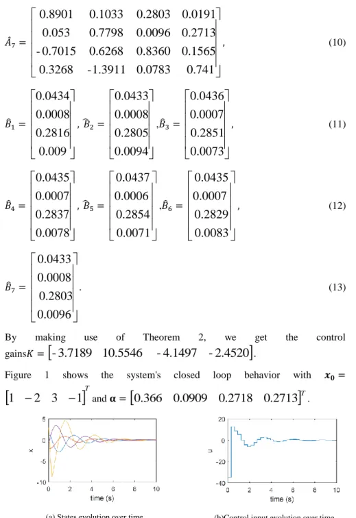
By making use of Theorem 2, we get the control gains𝐾 =
- 3.7189 10.5546 - 4.1497 - 2.4520
.Figure 1 shows the system's closed loop behavior with 𝒙𝟎=
1 2 3 1
Tand 𝛂 = 0.366 0.0909 0.2718 0.2713
T.(a) States evolution over time
(b)Control input evolution over time Figure 1
Closed loop behavior for the system in example 1
Example 2: Consider the 2 vertices system given in [28], described by 𝑥̇ = ∑2𝑖=1α𝑖(𝐴𝑖𝑥 + 𝐵𝑖𝒖).
with
𝐴1=
15 . 2 1 . 3
8 . 0 8 .
1
, 𝐴2=
01 . 3 34 . 4
12 . 1 a
𝐵1=
8 . 1
27 .
0
, 𝐵2 =
4 . 2
b
The aim of this example is to search the parameter space of a and b and find the region under which we are able to find a stabilizing controller. We compare the region found with the one in [28] with l = 5. We make use of 100 sample points for α1. We can see, from Figure 2, that, even though we make use of a simple condition, we are able to get better results than the ones in [28] with 𝑙 = 5.
Figure 2
Stabilizable region for the a and b parameters in example 2. The asterisks determine the stabilizable region for [28] with a fifth order truncation. The asterisks and dots represent the region stabilizable for
[28] with a fifth order truncation and linear search on the LMI conditions. The asterisks, dots and circles region represent the region stabilizable with the approach presented in this paper.
Conclusions and future works
This work proposed the use of the tensor product model transformation to approximate the matrix exponential function and find approximate uncertain discrete-time models for continuous-time uncertain systems with polytopic uncertainty. From the examples presented, we can see that the proposed methodology is a viable option, and allows the use of simpler LMIs for controller synthesis.
In the future, we aim to derive upper bounds on the approximation error during the sampling step of the tensor product model transformation and to make use of this upper bound in the control design in order to guarantee the continuous-time system stability when controlled by a digital controller tuned using the discrete- time model.
Referências
[1] Y. Nesterov and A. Nemirovskii, Interior-Point Polynomial Algorithms in Convex Programming. Society for Industrial and Applied Mathematics, 1994
[2] S. Boyd, L. E. Ghaoui, E. Feron, and V. Balakrishnan, Linear Matrix Inequalities in System and Control Theory. Society for Industrial and Applied Mathematics (SIAM), 1994
[3] N. Vlassis and R. Jungers, “Polytopic uncertainty for linear systems: New and old complexity results,” Systems & Control Letters, Vol. 67, pp. 9-13, 2014
[4] T. Chen and B. A. Francis, Optimal Sampled-Data Control Systems.
London, UK: Springer-Verlag, 1995
[5] S. Hara, Y. Yamamoto, and H. Fujioka, “Modern and classical analysis/synthesis methods in sampled-data control — A brief overview with numerical examples,” Proceedings of the 35th IEEE Conference on Decision and Control, Kobe, Japan, December 1996, pp. 1251-1256 [6] P. Blackmore, D. Williamson, and I. Mareels, “Open-loop discretization
methods for control systems design,” International Journal of Control, Vol.
74, No. 15, pp. 1527-1542, 2001
[7] T. Ono, T. Ishihara, and H. Inooka, “Design of sampled-data critical control systems based on the fast-discretization technique,” International Journal of Control, Vol. 75, No. 8, pp. 572-581, 2002
[8] L. S. Shieh, W. Wang, and G. Chen, “Discretization of cascaded continuous-time controllers and uncertain systems,” Circuits, Systems and Signal Processing, Vol. 17, No. 5, pp. 591-611, October 1998
[9] L. Hetel, J. Daafouz, and C. Iung, “LMI control design for a class of exponential uncertain systems with application to network controlled switched systems,” American Control Conference, New York, NY, USA, July 2007, pp. 1401-1406
[10] M. V. Kothare, V. Balakrishnan, and M. Morari, “Robust constrained model predictive control using linear matrix inequalities,” Automatica, Vol.
32, No. 10, pp. 1361-1379, October 1996
[11] S. Lee and S. Won, “Model Predictive Control for linear parameter varying systems using a new parameter dependent terminal weighting matrix,”
IEICE Transactions on Fundamentals of Electronics, Communications and Computer Sciences, Vol. E89-A, No. 8, pp. 2166-2172, 2006
[12] N. Wada, K. Saito, and M. Saeki, “Model predictive control for linear parameter varying systems using parameter dependent Lyapunov function,”
The 2004 47th Midwest Symposium on Circuits and Systems, Vol. 53, No.
12, pp. 1446-1450, December 2006
[13] M. Jungers, R. C. L. F. Oliveira, and P. L. D. Peres, “MPC for LPV systems with bounded parameter variations,” International Journal of Control, Vol. 84, pp. 24-36, January 2011
[14] M. F. Braga, C. F. Morais, E. S. Tognetti, R. C. L. F. Oliveira, and P. L. D.
Peres, “Discretisation and control of polytopic systems with uncertain sampling rates and network-induced delays,” International Journal of Control, Vol. 87, No. 11, pp. 2398-2411, November 2014
[15] F. Amato, M. Mattei, and A. Pironti, “A note on quadratic stability of uncertain linear discrete-time systems,” IEEE Transactions on Automatic Control, Vol. 43, No. 2, pp. 227-229, February 1998
[16] M. C. de Oliveira, J. Bernussou, and J. C. Geromel, “A new discrete-time robust stability condition,” System & Control Letters, Vol. 37, No. 4, pp.
261-265, July 1999
[17] M. C. de Oliveira, J. C. Geromel, and J. Bernussou, “Extended H2 andH1 characterization and controller parametrizations for discrete-time systems,”
International Journal of Control, Vol. 75, No. 9, pp. 666-679, June 2002 [18] G. Garcia, B. Pradin, S. Tarbouriech, and F. Zeng, “Robust stabilization
and guaranteed cost control for discrete-time linear systems by static output feedback,” Automatica, Vol. 39, No. 9, pp. 1635-1641, September2003 [19] M. C. de Oliveira, R. C. L. F. Oliveira, and P. L. D. Peres, “A new method
for robust Schur stability analysis,” International Journal of Control, Vol.
83, No. 10, pp. 2181-2192, October 2010
[20] K. J. A° stro¨m and B. Wittenmark, Computer Controlled Systems: Theory and Design. Englewood Cliffs, NJ: Prentice Hall Inc., 1984
[21] Y. Yam, P. Baranyi, and C.-T. Yang, “Reduction of fuzzy rule base via singular value decomposition,” IEEE Transactions on Fuzzy Systems, Vol.
7, No. 2, pp. 120-132, 1999
[22] P. Baranyi, D. Tikk, Y. Yam, and R. J. Patton, “From differential equations to PDC controller design via numerical transformation, ”Computers in Industry, Vol. 51, No. 3, pp. 281-297, 2003
[23] P. Baranyi, Y. Yam, and P. V´arlaki, Tensor Product Model Transformation in Polytopic Model-Based Control. Boca Raton, FL: CRCPress - Taylor &
Francis, 2013
[24] L. De Lathauwer, B. De Moor, and J. Vandewalle, “A Multilinear Singular Value Decomposition,” SIAM Journal on Matrix Analysis and Applications, Vol. 21, No. 4, p. 1253, 2000
[25] P. Varkonyi, D. Tikk, P. Korondi, and P. Baranyi, “A new algorithm for RNO-INO type tensor product model representation,” in 2005 IEEEInternational Conference on Intelligent Engineering Systems, INES’05. IEEE, 2005, pp. 263-266
[26] P. Baranyi, “Output feedback control of 2-d aeroelastic system, ”Journal of Guidance, Control, and Dynamics, Vol. 29, No. 3, pp. 762-767, 2006 [27] V. C. S. Campos, F. Souza, L. A. B. Tôrres, and R. M. Palhares, “New
stability conditions based on piecewise fuzzy Lyapunov functions and tensor product transformations,” IEEE Transactions on Fuzzy Systems, Vol. PP, No. 99, pp. 1-1, 2013
[28] M. F. Braga, C. F. Morais, E. S. Tognetti, R. C. L. F. Oliveira, and P. L. D.
Peres, “A new procedure for discretization and state feedback control of uncertain linear systems,” in 52nd IEEE Conference on Decision and Control, Dec 2013, pp. 6397-6402
[29] J. Löfberg, “YALMIP: A toolbox for modeling and optimization in MATLAB,” in Proceedings of the CACSD Conference, Taipei, Taiwan, 2004
[30] P. Baranyi: „TP-Model Transformation-Based-Control Design Frameworks”, Springer International Publishing Switzerland, 2016, p. 258 (eBook 978-3-319-19605-3, 978-3-319-19604-6, doi: 10.1007/978-3-319- 19605-3, http://www.springer.com/gp/book/9783319196046)
[31] A. Szollosi, P. Baranyi Influence of the Tensor Product Model Representation Of QLPV Models on The Feasibility of Linear Matrix Inequality, Asian Journal of control, 2016, pp 1328-1342
[32] A. Szollosi, and P. Baranyi, Improved control performance of the 3-DoF aeroelastic wing section: a TP model based 2D parametric control performance optimization, Asian Journal of Control, Vol. 19, number 2, pp 450-466, 2017
[33] A Szollosi, P. Baranyi „Influence of the Tensor Product Model Representation of qLPV Models on the Feasibility of Linear Matrix Inequality Based Stability Analysis”, Asian Journal of Control, 2017 in print