Tensor Product Model Transformation
Simplification of Takagi-Sugeno Control and Estimation Laws – An Application to a
Thermoelectric Controlled Chamber
Alisson Marden Fonseca Pereira, Letícia Maria Sathler Vianna, Natália Augusto Keles, Víctor Costa da Silva Campos
Departamento de Engenharia Elétrica, Instituto de Ciências Exatas e Aplicadas (ICEA), Universidade Federal de Ouro Preto (UFOP), Rua Trinta e Seis, 115, CEP 35931-008, João Monlevade/MG, Brazil, victor.campos@deelt.ufop.br
Abstract: This paper presents a novel application of the Tensor Product Model Transformation: the approximation of fuzzy control and estimation laws. In order to illustrate this application, a thermoelectric controlled chamber was built using peltier coolers and an H Bridge. Using 5 digital temperature sensors, a Takagi-Sugeno discrete time fuzzy model of the system was found with system identification techniques. A control and an estimation law were designed using state of the art LMI conditions for fuzzy systems. Making use of the Tensor Product Model Transformation, these control and estimation laws were approximated/simplified and implemented on a microcontroller. The results obtained from these simplified laws show that this is a viable option and allows the use of cheap microcontrollers in cases where it would not be able to implement the control and estimation laws.
Keywords: Tensor Product Model Transformation; Hinf model reference control; Takagi- Sugeno observer; LMI
1 Introduction
Takagi-Sugeno (TS) fuzzy systems [1] are widely studied due to their universal approximation capabilities. In addition, given the fact that they are capable of representing nonlinear systems by a convex combination of linear models, many control, estimation and analysis problems can be recast as Linear Matrix Inequality (LMI) problems [2-6].
The Tensor Product (TP) Model Transformation [7-11] is a numerical procedure that extracts a polytopic representation from a Linear Parameter Varying (LPV) one. This representation is equivalent to a TS fuzzy representation [8] and allows
the use of many TS analysis and synthesis conditions for these systems [9]. By doing so, it presents an alternative to the use of the sector nonlinearity approach [2] and automates the process by means of sampling, the Higher Order Singular Value Decomposition (HOSVD) and convex hull manipulations. In addition, it can also be used to reduce the number of rules in a TS model [11].
In this paper, we present a novel application of the TP model transformation under the TS LMI framework: the simplification of the control and estimation laws. In order to illustrate its effectiveness, a thermoelectric heating/cooling system is designed and implemented using Peltier effect. Two Thermoelectric coolers (TECs) modules are used to change the temperature inside of a chamber made out of wood and styrofoam. In order to ensure that the system could be controlled, a power circuit is built in such a way that the polarity and the level of the voltage applied to the TEC modules could be easily changed.
In order to find suitable control and estimation laws for the system, system identification techniques are employed to retrieve a discrete-time TS model of the system. In possession of this model, the control and estimation laws are found from suitable LMI conditions and the TP model transformation is used to simplify these laws in a way that they can be implemented in real-time.
The structure of this paper is as follows. Section 2 presents the system used to illustrate the paper’s main idea. Section 3 presents the system’s model identification. Section 4 shows the conditions required to design the control law.
Section 5 presents the conditions required to synthesize the fuzzy observer.
Section 6 presents the idea of approximating control and estimation laws through tensor product model transformation. Section 7 presents this works conclusions.
Notation Throughout this paper, scalars are represented by lowercase variables, column vectors by lowercase boldface variables, matrices by uppercase variables and tensors by calligraphic uppercase variables. 𝐴𝑇 denotes the transpose of 𝐴, 𝑃 > 0 (𝑃 ≥ 0) indicates that matrix 𝑃 is positive definite (semi-definite), and
∗represents symmetric terms inside of a symmetric matrix. 𝒮 ×𝑛𝑈 represents the n-mode product between tensor 𝒮 and matrix𝑈.𝒮 ⊠i=1n 𝑈𝑖 is a shorthand notation for 𝒮 ×1𝑈1… ×𝑛𝑈𝑛. 𝐴 ⊗ 𝐵 denotes the Kronecker product between 𝐴 and 𝐵.𝐴ℎ
is a shorthand notation for ∑𝑟𝑖=1ℎ𝑖(𝑥𝑘)𝐴𝑖, and 𝐴ℎ− is a shorthand notation for
∑𝑟𝑖=1ℎ𝑖(𝑥𝑘−1)𝐴𝑖.
2 Thermoelectric Cooler-based Chamber
Cooling systems based on Peltier modules have the advantage of being much more environmentally friendly compared to conventional refrigerators which, despite superior performance, release gas into the environment. The operating temperature range inside the built chamber can be varied from 16 to 40 degrees Celsius.
The chamber is 40 centimeters of length and 30 centimeters of width and height.
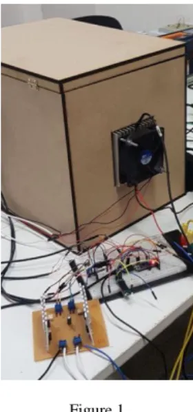
Two 100 cm2 square holes were opened to accommodate two structures, each containing one Peltier module TEC 12715, two heat sinks and two fans. The Peltier module is placed between the two heat sinks, which are responsible for increasing the superficial area of the Peltier module and thus increase the heat transfer. The remaining air gap is filled with pieces of Styrofoam. The fans spread the heat uniformly. Figure 1 shows the final version of the chamber.
Figure 1 Thermoelectric chamber
We simplify the system’s representation (to a lumped parameter one) and consider that its dynamics can be represented by five different temperatures: two on the external heat sinks, two on the internal heat sinks and one in the middle of the chamber. In order to measure these temperatures, five digital sensors were used, specifically DS18B20 sensors, which were configured to have an accuracy of 0.0625 °C.
The two TECs were connected in series and powered by a MOSFET H-Bridge so that they could be used to either cool or heat the chamber. A microcontroller was used to sample the sensor measurements and generate the PWM signals for the H- Bridge.
3 Takagi-Sugeno System Identification
Throughout this paper, we consider that the system is described by a discrete-time TS model given by
𝒙𝑘+1= ∑𝑟𝑖=1ℎ𝑖(𝒙𝑘)(𝐴𝑖𝒙𝑘+ 𝐵𝑖𝒖𝑘)= 𝐴ℎ𝒙𝑘+ 𝐵ℎ𝒖𝑘, (1)
𝑦𝑘 = 𝐶𝒙𝑘. (2) Note that, if the membership functions are fixed and all states are measured (as we consider in this paper) this model is linear in the parameters and can be rewritten as
𝒙𝑘+1= [𝐴1 𝐵1 ⋯ 𝐴𝑟 𝐵𝑟] (𝒉(𝒙𝒌) ⊗ [𝒙𝒌
𝒖𝑘]) (3)
𝒙𝑘+1= (𝒉𝑻(𝒙𝒌) ⊗ [𝒙𝒌𝑻 𝒖𝒌𝑻]) [ 𝑨𝟏𝑻
𝑩𝟏𝑻 𝑨⋮𝒓𝑻 𝑩𝒓𝑻]
(4)
In this case, by making use of input and output data, we can make use of the Least Squares Method [1] and find a TS model as in (1).
For the Thermoelectric chamber, we consider that the left external temperature is the first state, the left internal temperature is the second state, the right internal temperature is the third state, the right external temperature is the fourth state and that the temperature in the middle of the chamber is the fifth state. We made use of a random input signal ranging from 0 to 12 V, shown in Figure 2, and measured the five states using the available sensors, shown in Figures 3 to 5.
Figure 2
Input data used for the system identification
In this application case, we considered that the only premise/scheduling variable is the temperature in the middle of the chamber and we made use of a Takagi- Sugeno model with 13 rules and gaussian membership functions. We considered 16.6, 18.73, 20.87, 23, 25.13, 27.27, 29.4, 31.53, 33.67, 35.8, 37.93, 40.07 and
42.2 as the mean and 0.71 as the standard deviation for the gaussian membership functions. The resulting normalized membership functions are shown in Figure 6.
For the sake of comparison, Figure 7 shows, for a different set of input and output data, the measured temperatures in the middle of the chamber together with a free run simulation of the TS model found.
Figure 3
Temperature on the chamber’s external heat sinks
Figure 4
Temperature on the chamber’s internal heat sinks
Figure 5
Temperature in the middle of the chamber
Figure 6
Membership functions used in the example
Figure 7
Temperature on the middle of the chamber – real vs. simulated
4 𝓗
∞Model Reference PDC Control Law
In order to design a controller capable of reference tracking with a behavior close to a desired one, we make use of a ℋ∞model reference approach.
With a small notational abuse, Figure 8 presents a block diagram of this approach.
In this Figure, 𝐻(𝑧) represents a discrete-time TS fuzzy model (as in (1)), 𝐻𝑚(𝑧) represents a desired model for the system, and 𝑧
𝑧−1 represents a discrete-time integrator (used to ensure that there will not be any steady state errors between the system and the reference model). In this setting, we aim to find an ℋ∞ controller that minimizes the gain from the reference of the desired model to the integral of the error between the two models.
Figure 8
Open Loop Block Diagram for the ℋ∞ model reference control approach If we consider a linear reference model given by
𝒙𝑚𝑘+1= 𝐴𝑚𝒙𝑘+ 𝐵𝑚𝒓𝒌, (5)
𝑦𝑚𝑘= 𝐶𝑚𝒙𝒌, (6) We can represent the desired block diagram as the augmented system
[ 𝒙𝑘+1
𝒙𝒎𝑘+1
𝒍𝑘+1 ] = [
𝐴ℎ 0 0
0 𝐴𝑚 0
𝐶 −𝐶𝑚 𝐼] [ 𝒙𝑘
𝒙𝒎𝑘
𝒍𝑘 ] + [𝐵ℎ 0 0
] 𝒖𝑘+ [0 𝐵𝑚
0
] 𝒓𝑘, (7)
𝒛𝑘 = [0 0 𝐼] [ 𝒙𝑘 𝒙𝑚𝑘
𝒍𝑘
]. (8)
A shorter representation for the augmented system is given by
𝒙̅𝑘+1= 𝐴̅ℎ𝒙̅𝑘+ 𝐵̅ℎ𝒖𝑘+ 𝐵̅𝑟𝒓𝑘, (9)
𝒛𝑘 = 𝐶̅𝒙̅𝑘, (10)
with 𝒙̅𝑘= [𝒙𝑘𝑇 𝒙𝑚𝑇𝑘 𝑙𝑘𝑇]𝑇, 𝐴̅ℎ = [
𝐴ℎ 0 0
0 𝐴𝑚 0
𝐶 −𝐶𝑚 𝐼], 𝐵̅ℎ = [𝐵ℎ
0 0
] , 𝐵̅𝑟= [ 0 𝐵𝑚
0 ], and 𝐶̅ = [0 0 𝐼].
From the literature [6], we know that, considering a control law, with delayed membership functions, of the form
𝒖𝑘 = 𝐾ℎℎ−𝐺ℎℎ −1−𝒙̅̅̅, 𝑘 (11) a sufficient condition for
||𝑧||2
||𝑤||2 ≤ 𝛾, (12)
is that there exist matrices 𝑃𝑖, with 𝑖 ∈ {1,2, … , 𝑟}, and 𝐾𝑖𝑗 and 𝐺𝑖𝑗, with 𝑖, 𝑗 ∈ {1,2, … , 𝑟}, such that
∑ ∑ ∑
𝑟𝑖=1 𝑟𝑗=1 𝑟𝑙=1ℎ𝑖(
𝒙𝑘)
ℎ𝑗(𝒙𝑘)ℎ𝑙(
𝒙𝑘−1)
𝑄𝑖𝑗𝑙 < 0, (13) with𝑄𝑖𝑗𝑙 =
[
−𝐺𝑗𝑙𝑇 − 𝐺𝑗𝑙+ 𝑃𝑙
∗∗
∗
0
−𝛾𝐼
∗
∗
𝐺𝑗𝑙𝑇𝐴
̅
𝑖𝑇+ 𝐾𝑗𝑙𝑇𝐵̅
𝑖𝑇𝐵
̅
𝑚𝑇−𝑃𝑖
∗
𝐺𝑗𝑙𝑇𝐶
̅
𝑇00
−𝛾𝐼
]
. (14)In order to implement this set of parameter-dependent LMIs, we make use of the following sufficient conditions
𝑄𝑖𝑖𝑙< 0 ∀ 𝑖, 𝑙, (15)
𝑄𝑖𝑗𝑙+ 𝑄𝑗𝑖𝑙 < 0 ∀𝑖, 𝑗 > 𝑖, 𝑙. (16)
Since we are dealing with a real physical system, and ℋ∞ controllers tend to have very large gains, we also make use of a set of limiting conditions for the controller gains. By making use of the S-procedure, it is easy to see that if there exists 𝜏 ∈ ℝ such that
[
−𝐺𝑖𝑗𝑇 − 𝐺𝑖𝑗
∗∗
∗
0
−𝛿
𝑢2+ 𝛿
𝑥2𝜏∗
∗
𝐾
𝑖𝑗𝑇−1 0
∗
𝐼
00
−𝜏𝐼
] < 0, ∀𝑖, 𝑗,
(17)then, the control law found is such that
𝒖𝑻𝒖 ≤ 𝜹𝒖𝟐, ∀𝒙𝑻𝒙 ≤ 𝜹𝒙𝟐. (18)
5 Fuzzy State Observer with Measurable Premisse Variables
In many practical applications, the states of a given system are not always readily available. Therefore, given the output measurements and the system’s input, a state observer can be used to estimate the system’s state. In this work, we consider the particular case in which all of the premise variables are measured, and search for the TS observer with the highest decay rate possible.
Considering a TS model described by (1) and (2), we consider a fuzzy observer with measurable premise variables given by
𝒙̂𝒌+𝟏= 𝑨𝒉𝒙̂𝒌+ 𝑩𝒉𝒖𝒌+ 𝑴𝒉−𝟏−𝑵𝒉𝒉−(𝒚𝒌− 𝒚̂𝒌). (19)
𝒚̂𝒌+𝟏 = 𝑪𝒙̂𝒌. (20)
with 𝑀ℎ− and 𝑁ℎℎ− the observer gains.With this observer, the estimation error, 𝒆𝒌= 𝒙𝒌− 𝒙̂𝒌, dynamics is given by
𝒆𝒌+𝟏= (𝐴ℎ− 𝑀ℎ−1−𝑁ℎℎ−𝐶)𝒆𝒌. (21)
As shown in [12], by making use of a Lyapunov function with delayed membership function,
𝑽𝒌= 𝒆𝒌𝑃ℎ−𝒆𝒌, (22)
the system is asymptotically stable if there exist matrices 𝑃𝑖 and 𝑀𝑖 with 𝑖 ∈ {1,2, … , 𝑟}, and 𝑁𝑖𝑗 with 𝑖, 𝑗 ∈ {1,2, … , 𝑟} such that
[−𝑷𝒊 𝑨𝒊𝑻𝑴𝒋𝑻+ 𝑪𝑻𝑵𝒊𝒋𝑻
∗ −𝑮𝒋𝑻− 𝑮𝒋+ 𝑷𝒋] < 0. (23)
In addition to this, if the Lyapunov function is such that
𝑽𝒌+𝟏< 𝜶𝟐𝑽𝒌, (24) then the system will be exponentially stable with a decay rate of 𝛼. It is easy to show that, in the case of the LMI conditions presented above, this amounts to [−𝜶𝟐𝑷𝒊 𝑨𝒊𝑻𝑴𝒋𝑻+ 𝑪𝑻𝑵𝒊𝒋𝑻
∗ −𝑮𝒋𝑻− 𝑮𝒋+ 𝑷𝒋] < 0. (25)
6 Control and Estimation Laws Simplification
Having found the control and estimation gains, and remembering the fact that the separation principle is still valid when we use a fuzzy observer with measurable premise variables [2], we can use them together to form an output feedback control law for the system. In this case, the controller dynamics can be written as 𝒖𝑘 = 𝐾ℎℎ−𝐺ℎℎ −1−[𝒙̂𝒌𝑻 𝒙𝑚𝑇𝑘 𝒍𝑘𝑇]𝑇,(26)
𝒙̂𝒌+𝟏= (𝐴ℎ− 𝑀ℎ−1−𝑁ℎℎ−𝐶)𝒙̂𝒌+ 𝐵ℎ𝒖𝒌+ 𝑀ℎ−1−𝑁ℎℎ−𝒚𝒌, (27)
𝒙𝑚𝑘+1= 𝐴𝑚𝒙𝑘+ 𝐵𝑚𝒓𝒌, (28)
𝒍𝑘+1= −𝐶𝑚𝒙𝑚𝑘+ 𝒍𝑘+ 𝒚𝒌. (29)
Notice that these equations are rather complicated to implement in real time on a microcontroller since the inverses 𝐺ℎℎ −1−and 𝑀ℎ−1− need to be calculated in real time.
A possible approach to circumvent this issue is to make use of the TP model transformation to approximate the control and estimation gains.
In that regard, consider a parameter varying matrix defined by 𝑆ℎℎ−= [𝐴ℎ 𝐵ℎ 𝑀ℎ−1−𝑁ℎℎ−
𝐾ℎℎ−𝐺ℎℎ −1− 0 ]. (30)
we may define a sampling grid over the current and past fuzzy premise variables and apply the Tensor Product Model Transformation to this parameter varying matrix.
One could argue that, in this case, we could just use the HOSVD step to reduce the control and estimation gains complexity since this particular TP model will not be used on a further LMI design step. Note, however, that the weights found from the HOSVD step may have any value, and as such make it hard to interpret the gains found. In that regard, it is advisable to make use of the convex hull manipulation step, preferably with a tighter transformation (like the Close to Normalized – CNO [13]), so that we can make sense of the control and estimation gains found.
It is important to note that, even though the choice of the convex hull transformation can be a decisive factor on whether or not an LMI synthesis
procedure is successful [14-16], they do not affect the feasibility of the LMIs in the strategy proposed in this paper (as they are used simply with the control and estimation laws as opposed to finding a convex representation used in the LMIs).
Nevertheless, it is recommended to use the CNO transformation, as it will lead to control and estimation gains that can be more easily interpreted.
For the thermoelectric controlled chamber, since we are only using the middle temperature as a premise variable, the parameter varying matrix 𝑆ℎℎ− depends only on the current and one step past values of this premise variable. In that regard, we consider a 2-dimensional grid for these values, with 40 points in each direction.
In addition to this, we consider that there is a single control input; the desired controlled temperature is the one on the middle of the chamber, only the middle temperature and one of the external heat sinks’ temperatures are measured, and we consider a stable linear reference model with a single state. With all of these considerations, we have that 𝑆ℎℎ−∈ ℝ6×8 and we store the sampled matrices on a 𝒮 ∈ ℝ40×40×6×8 tensor.
Due to the microcontroller memory limitations, in the HOSVD step we keep only 3 columns, corresponding to the 3 highest singular values, in each of the 2 first directions. However, when making use of the convex hull manipulations, a fourth column was added in each direction, resulting in an equivalent fuzzy TP model with 16 rules (4 × 4).
By making use of triangular membership functions and a uniform grid distribution, it is easy to show that there exists an efficient (𝑂(1)) linear interpolation scheme to implement the control and estimation membership functions, which justifies the use of the Tensor Product Model Transformation as an efficient way to implement the control and estimation laws.
For comparison purposes, Figures 9 and 10 present the membership functions found for the current and past middle temperature in the control and estimation laws. Note their difference from the original membership functions presented in Figure 6.
Figure 9
Control and Estimation membership functions found after the TP model transformation for the current value of the middle temperature
Figure 10
Control and Estimation membership functions found after the TP model transformation for the previous value of the middle temperature
The system’s behavior in closed loop with the approximate control and estimation laws can be seen on Figures 11 to 17. Figure 11 presents the controlled temperature against its desired values, Figure 12 presents the calculated control input and the actual control input applied to the systems, whereas Figures 13 to 17 present the estimates found for the five temperatures against their measured values.
Figure 11
Controlled temperature inside of the chamber together with the desired reference model output and the desired temperature reference
Figure 12
Calculated control input over time with the control input that was actually applied to the sysstem
Figure 13
Estimated and measured temperatures on the left external heat sink. The red line represents the measured values, whereas the blue one represents the estimated one
Figure 14
Estimated and measured temperatures on the left internal heat sink. The red line represents the measured values, whereas the blue one represents the estimated one
Figure 15
Estimated and measured temperatures on the right internal heat sink. The red line represents the measured values, whereas the blue one represents the estimated one
Figure 16
Estimated and measured temperatures on the right external heat sink. The red line represents the measured values, whereas the blue one represents the estimated one
Figure 17
Estimated and measured temperatures on the middle of the chamber. The red line represents the measured values, whereas the blue one represents the estimated one
Conclusions
This paper presented a novel application to the tensor product model transformation, specifically its use on the approximation and simplification of fuzzy control and estimation laws. The proposed methodology was applied to a thermoelectric controlled chamber and yielded satisfactory results.
Future works on this line will focus on the development of non-fragile controller and estimation conditions that are guaranteed to work even when there’s a mismatch between the designed and the implemented control and estimation gains.
References
[1] Takagi, T., & Sugeno, M. (1985) Fuzzy identification of systems and its applications to modeling and control. IEEE transactions on systems, man, and cybernetics (1) 116-132
[2] Tanaka, Kazuo; Wang, Hua O. Fuzzy control systems design and analysis:
a linear matrix inequality approach. John Wiley & Sons, 2004
[3] Guerra, Thierry-Marie et al. An efficient Lyapunov function for discrete T–
S models: observer design. IEEE Transactions on Fuzzy Systems, v. 20, n.
1, pp. 187-192, 2012
[4] Tanaka, Kazuo; Ikeda, Takayuki; Wang, Hua O. Fuzzy regulators and fuzzy observers: relaxed stability conditions and LMI-based designs. IEEE Transactions on fuzzy systems, v. 6, n. 2, pp. 250-265, 1998
[5] Estrada-Manzo, Victor; Lendek, Zsófia; Guerra, Thierry Marie.
Generalized LMI observer design for discrete-time nonlinear descriptor models. Neurocomputing, v. 182, pp. 210-220, 2016
[6] Lendek, Z., Guerra, T. M., & Lauber, J. (2015) Controller design for TS models using delayed nonquadratic Lyapunov functions. IEEE Transactions on Cybernetics, 45(3) 439-450
[7] Yam, Y., Baranyi, P., & Yang, C. T. (1999) Reduction of fuzzy rule base via singular value decomposition. IEEE Transactions on fuzzy Systems, 7(2) 120-132
[8] Baranyi, P., Tikk, D., Yam, Y., & Patton, R. J. (2003) From differential equations to PDC controller design via numerical transformation.
Computers in Industry, 51(3) 281-297
[9] Baranyi, P. (2004) TP model transformation as a way to LMI-based controller design. IEEE Transactions on Industrial Electronics, 51(2) 387- 400
[10] Baranyi, P., Yam, Y., &Várlaki, P. (2013) Tensor product model transformation in polytopic model-based control. CRC Press
[11] Campos, V. C. S., Tôrres, L. A. B., & Palhares, R. M. (2015) Revisiting the TP model transformation: Interpolation and rule reduction. Asian Journal of Control, 17(2) 392-401
[12] Guerra, T. M., Kerkeni, H., Lauber, J., & Vermeiren, L. (2012) An efficient Lyapunov function for discrete T–S models: observer design. IEEE Transactions on Fuzzy Systems, 20(1) 187-192
[13] Campos, V. C., Souza, F. O., Tôrres, L. A., & Palhares, R. M. (2013) New stability conditions based on piecewise fuzzy Lyapunov functions and tensor product transformations. IEEE Transactions on Fuzzy Systems, 21(4) 748-760
[14] Szollosi, A., & Baranyi, P. (2016) Influence of the Tensor Product model representation of qLPV models on the feasibility of Linear Matrix Inequality. Asian Journal of Control, 18(4) 1328-1342
[15] Baranyi, P. (2014) The generalized TP model transformation for T–S fuzzy model manipulation and generalized stability verification. IEEE Transactions on Fuzzy Systems, 22(4) 934-948
[16] Gróf, P., Baranyi, P., &Korondi, P. (2010) Convex hull manipulation does matter in LMI based observer design, a TP model transformation based optimisation. strategies, 11, 12