Continuous time Robust Fixed Point Transformations based control
Bence G´eza Czak´o1, D´aniel Andr´as Drexler1 and Levente Kov´acs1
Abstract— The Robust Fixed Point Transformation based control proved to be beneficial in controlling nonlinear systems with structural or parametric discrepancies. The method was originally formalized in discrete time, using local deformations to alter the input trajectory in order to diminish the uncertain- ties. A continuous time counterpart is introduced in this paper, which also connects the method to the feedback linearization principle. Such a formalism should make it possible for one to use tools from the classical continuous time literature to analyse the properties and convergence of the method. The theory is demonstrated by controlling angiogenic inhibition of tumor growth using the minimal model.
I. INTRODUCTION
Input-output (feedback) linearization is a powerful tool in the synthesis of nonlinear controllers. Since its development in the 1980’s, many applications showed its effectiveness in treating nonlinearities, where conventional linear techniques might be inadequate. The underlying idea of the technique is that by finding a proper transformation of the original nonlinear system, the input signal can be chosen such that it cancels out the nonlinearities; rendering the system into a purely linear system [1]. This linear system can be controlled by conventional techniques, pole placement or integrating path tracking control (ITC) for example.
While the technique is one of the most popular design methodology in nonlinear control, it has a few disadvantages as well. Two such problems include the treatment of zero dynamics and the handling modelling uncertainties, from which this paper focuses on the latter. While the issue of zero dynamics has been widely researched in the past decades, robustness of uncertainties has not gained such a significant attention according to [2]. Results concerning parametric uncertainties can be found in the adaptive control literature, where the controller design usually relies on the utilization of Lyapunov functions [3], [4]. While stability of the system can be guaranteed in such a way, the design procedure might be cumbersome in systems where it is nontrivial to find a proper Lyapunov function.
Over the past decade a novel approach called Robust Fixed Point Transformation (RFPT) based control method
This project has received funding from the European Research Council (ERC) under the European Union’s Horizon 2020 research and innovation programme (grant agreement No 679681). Bence G. Czak´o was supported by the UNKP-18-3/II. New National Excellence Program of the Ministry of Human Capacities
The Authors are with the Physiological Controls Research Center within the Research, Innovation and Service Center of Obuda University, Budapest, Hungary czako.bence@phd.uni-obuda.hu drexler.daniel@nik.uni-obuda.hu
kovacs@uni-obuda.hu
was introduced by Tar et al., which relies on a numerical treatment of the problem using fixed point iterations to solve the control task [5], [6]. If one is able to establish a nominal model for the plant, an approximate inverse can be carried out, which is then can be used to calculate the input signal for a certain trajectory. However, if there is a significant structural or parametric discrepancy between the nominal model and the plant, the resulting input signal will not be able to steer the system along the desired trajectory. The underlying idea is to deform the reference trajectory so that the inverse model produces the proper input signal for the plant. The modified reference trajectory was calculated using deform functions, that are, specific root finding algorithms with enhanced convergence properties that are suitable for wide classes of nonlinear models arising in control problems.
One enormous benefit of the technique is that it gives a simple design procedure, bypassing the use of Lyapunov functions. Once one obtained an inverse model for the system to be controlled, a deform function must be chosen which is able to compute the reference trajectory. The control parameters in this case can be attributed to the deform function, and can be empirically set via multiple simulations.
Many practical application of the controller showed that one can obtain a very precise tracking, even in the presence of uncertainties [7], [8], [9], [10]. Despite of the obvious practical advantages, one must be aware that results con- cerning stability and robustness of the method has not been established due to its novelty. Rudimentary results can be found on stability and auto tuning, however, a more rigorous treatment must be developed in order to be a vastly applicable control technique [11], [12]. The aim of this paper is to formalize continuous counterpart of the discrete time RFPT by connecting it to the feedback linearization principle.
Section II introduces the basics of input-output linearization in the absence of zero dynamics. This is followed by the formulation of the RFPT technique by defining the error between the inverse model and the plant in Section III Section IV demonstrates an application of the method on a tumor volume regulation problem using the minimal model with an example of the robust behaviour of the controller [15].
II. INPUT-OUTPUT LINEARIZATION
In the section, a brief introduction is made to the input- output linearization principle, based on [1]. Consider the following input affine SISO nonlinear system:
˙
x=f(x) +g(x)u
y=h(x) (1)
wherex∈Rnis the state vector,u∈Ris the input, y∈Ris the output of the system, and f,g,h are sufficiently smooth vector fields. Differentiating the output leads to:
˙ y=∂h
∂xx˙=∂h
∂x[f(x) +g(x)u]Lfh+Lgh u (2) whereLfhandLghare the Lie derivatives ofh along f and g respectively. The notation has the following property:
L0fh=h
Lkfh=LfLk−1f h=∂(Lk−1f h)
∂x f
(3) Assume that the control input u only appears in the ρ-th derivative of the output, with the coefficient
LgLfh=∂(Lfh)
∂x g. (4)
The number ρ is called the relative degree of the system which is now defined.
Definition 1(Relative degree). The nonlinear system (1) has a relative degreeρ(1≤ρ≤n)in a region D0⊂D, if
LgLi−1f h(x) =0, i=1,..,ρ−1
LgLρ−1f h(x)=0 (5)
for all x∈D0.
If the relative degree is smaller than the dimension of the state vector, one must analyse the zero dynamics of the system. For a concise introduction, we assume that the relative degree is maximal i.e. ρ =n, so that the system does not admit zero dynamics. One can define the following coordinate transformation that renders the system into its normal form:
⎛
⎜⎜
⎜⎝ ξ1
ξ2
... ξρ
⎞
⎟⎟
⎟⎠=Φ(x) =
⎛
⎜⎜
⎜⎝ h(x) Lfh(x)
... Lρ−1f h(x)
⎞
⎟⎟
⎟⎠ (6)
whereΦ:Dx⊂Rn→Dξ⊂Rnmust be a differentiable and invertible map. The transformation is composed of the Lie derivatives of the output along f and leads to the following system:
ξ˙1=ξ2
ξ˙2=ξ3
... ξ˙ρ−1=ξρ
ξ˙ρ=α(ξ) +β(ξ)u
(7)
where the last equation contains the nonlinearities with:
α(ξ) = [Lρfh(x)]x=Φ-1(ξ)
β(ξ) = [LgLρ−1f h(x)]x=Φ-1(ξ) (8) This system contains an integrator series, which is purely linear, and a nonlinear expression in ˙ξρ. At this point one can choose the input signal to be:
u=r−α(x)
β(x) (9)
which cancels out the nonlinearities, leading to ˙ξρ=r, where r is a virtual input. An integrating path tracking controller (ITC) can be designed for such a system that ensures the error dynamics:
Λ+ d
dt
ρ+1 t 0
e(τ)dτ=0 (10) where Λ is a control parameter, e(t) =ξ¯1(t)−ξ1(t) with ξ¯1being the reference trajectory. From (10), we can express ξ1(ρ)which defines the control law of the ITC, i.e., the output uitc of the linear controller.Λ is a control parameter which must be chosen such that the Laplace transform of the time derivative of the error dynamics (10) is Hurwitz [13].
III. CONTINUOUS TIME RFPT
While the input-output linearization is a powerful concept, it suffers from the aforementioned robustness issue. For a brief introduction, we deal with parametric uncertainties exclusively, although practical examples revealed that the RFPT can deal with structural discrepancies as well [8]. We also assume, that the changes in the parameters do not affect the relative degree. Consider the nominal nonlinear system, in the same form as (1):
˙˜
x=f˜(x˜) +g˜(x˜)u
˜
y=h(˜ x)˜ (11)
where ˜f,g˜and ˜h are the known vector fields of the nominal model, that might differ from the original system only in their parameters, not necessarily linearly and ˜x is the state space variable of the nominal model. If one follows the process described in the previous section, a modified inverse model can be obtained, that is:
ϕ˜−1: u=uitc−Lρf˜h(x)˜
Lg˜Lρ−f˜ 1h˜(x) (12) Substituting this inverse into (7) results in:
y(ρ)=ξ˙ρ=Lρfh(x) +LgLρ−1f h(x)uitc−Lρf˜h˜(x) Lg˜Lρ−1˜
f h˜(x) (13) withϕ=Lρfh(x)+LgLρ−1f h(x). As one can see, this equation is a complicated nonlinear expression, which prevents the use of linear controllers. The goal is to force theρth derivative of the output y(ρ) to match exactly the ITC output uitc;
if the model is known exactly then this is carried out by the inverse dynamics (12). However, if the model is not known the inverse dynamics transformation cannot ensure this equivalence and we require a modified input ˜uitc. The control law is updated iteratively in order to approximate ˜uitc. This update is based on the inverse dynamics error defined by
einv=y(ρ)−uitc (14) wherey(ρ)is theρ-th order derivative of the real (measured) output which depends on the modified controller output that will be denoted by r and will be transformed to system input by (9). The naive approach would be to rearrange the equation algebraically, from which r can be computed analytically, although this is impossible in the vast majority of nonlinear systems. In this form, the problem is basically a root-finding problem onr, which entails that one can utilize a fixed point iteration to solve the equation. Fixed point iterations must be in the form of G(r) =r where G is the so called deform function, which leads to that (14) must be transformed into
y(ρ)−uitc+r=r. (15) where the virtual input r that satisfies (15) can be found as the fixed point of the iteration G(rn) =rn+1 with G being the left-hand side of (15). One major issue with (15) is the poor convergence property of the induced iteration because it is completely determined by the contractivity of the nonlinear operator and the reference trajectory [14].
In order to overcome this issue, the deform function G is modified to a form which is able to deal with a wide class of nonlinearities proposed by Tar et al. [6]:
G(r)(r+K)[1+Btanh(A[y(ρ)−uitc])]−K, (16) whence the iteration is achieved by G(rn) =rn+1 andK,A and B are control parameters with rn being the function r in then-th iteration. Based on the initial functionr0 and the value of the parametersK,AandB, three different scenarios might occur:
• The iteration does not converge, i.e., the mapping Gis not contractive.
• The iteration converges to the improper fixed point−K.
• The iteration converges to the proper fixed point r∗ which ensure that inverse dynamics error (15) is zero.
The outcome of the iteration can be modified by tuning the control parameters of the deform function, or by choosing a better initial guess r0. The ultimate goal is to obtain an attractive fixed point r∗ which is the modified virtual input. The convergence of the iteration can be analysed using the Banach fixed-point theorem, which is now stated in conjunction with the definition of contractivity [14]:
Definition 2 (k-contractivity). An operator G:M⊆X→X on a metric space (X,d)is called k-contractive on M if
d(Gx,Gy)≤kd(x,y) (17)
with fixed0≤k<1 and for all x,y∈M.
Theorem 1 (Banach Fixed-Point Theorem). If a given op- erator G:M⊆X→X is k-contractive on M then G admits a unique fixed point on M, i.e. G(r∗) =r∗, and r∗ can be obtained by successive iterations in the form if G(rn) =rn+1 for an arbitrary r0∈M.
In the case of RFPT,r∈M⊆X lies in the Banach space of Lebesgue measurable functions on a finite interval [0,t] with finite essential supremumX=L∞([0,t],R). According to Theorem 1, convergence of the iteration (16) can be assured by tuning the control parameters from which K is a large positive number, A is usually a small number with A=1/(10·K) and B is either 1 or −1. A suitable initial r0 must be chosen as well in order to obtain a fixed point by the iteration. One possible choice is to use input-output linearization to solve the control problem assuming that the nominal model is the same as the original and take the virtual input generated by the controller which then can be regarded asr0for the iteration in the RFPT method. A useful condition on contractivity on a finite interval is
||G(r)||<1, (18) which means that the derivative of the deform function on the whole range of r must be smaller than one, which can be ensured by the proper choice of the design parameters.
The proposed nonlinear controller can be seen in Fig. 1.
IV. RFPT CONTROL OF TUMOR GROWTH Consider the minimal model proposed by Drexler et al.
[15] which describes tumor growth under angiogenic inhibi- tion. The model is a simple two state SISO system as
˙
x1=ax1−bx1x2
x˙2=−cx2+u y=x1
(19)
where x1 is the tumor volume in mm3, x2 is the inhibitor level in the host measured in mg/kg,a is the tumor growth rate defined in 1/day, b is the inhibition rate given in kg / (mg·day) andc is the clearance of the inhibitor measured in 1/day. The exact model parameters are a=0.27, b= 0.0074 and c=ln(2)/3.9, identified by mice experiments.
The model has an unstable equilibrium atx1=x2=0 mm3 if no input is present. The aim is to control the size of the tumor, specifically, follow the trajectory defined as
x¯1=x1(0)exp(−t/100) (20) with derivatives for the kinematic block:
˙¯
xr1=−x1(0)10−2 exp(−t/100)
¨¯
xr1=x1(0)10−4exp(−t/100) (21) The first step in the controller design is to determine the relative order of the system. The Lie derivatives of 19 are
Fig. 1. The RFPT controller
Lfh=ax1−bx1x2 Lgh=0
L2fh=x1(a−bx2)2+bcx1x2
LgLfh=−bx1
(22)
whence the relative degree ρ=2, since the input explicitly appears in the second derivative of the output. The transfor- mation of the states is given by
ξ1
ξ2 =Φ(x) =
x1
ax1−bx1x2 (23) from which the system takes the form of
ξ˙1=ξ2
ξ˙2=x1(a−bx2)2+bcx1x2−bx1u (24) Thus, the inverse model of the system which renders it linear in an input-output sense is given by
u=r−x1(a−bx2)2+bcx1x2
−bx1 (25)
The next step is to design the ITC, which is determined by the relative degree of the system. Substitutingρ=2 into (10) and rearranging the terms leads to the following prescription on the virtual inputr:
Λ3 t1
t0
e(τ)dτ+3Λ2e(t) +3Λe˙(t) +x¨¯1=uitc (26) The deform function is the same as (16) with y(ρ)(r) =x¨1
with initial value r0 of the iteration that is uitc. Parameters were determined by numerical simulations empirically as K =107,A=10−8 and B=−1. Initial simulations were conducted on a 300 days interval, concerning the operation of the controller upon no parameter discrepancies. Multiple simulations suggested that approximately after 20 iterations the method converges and no further improvement can be made.
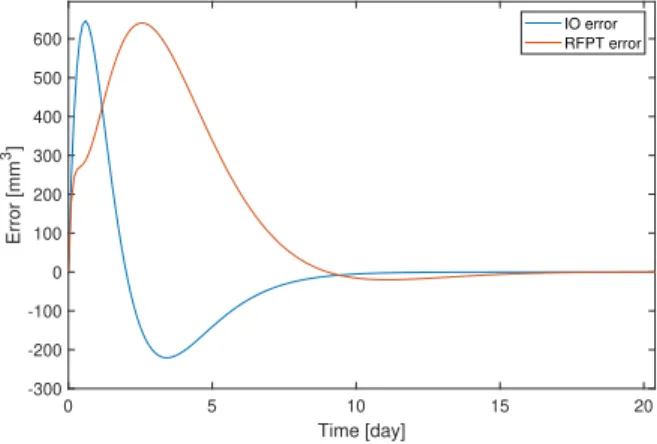
Fig. 2. shows the output of both the input-output lineariza- tion (IO) and the RFPT based controller. As one can see the difference between both trajectories are negligible which can be seen clearly from Fig. 3. Simulations also revealed that the integral of the RFPT tracking error is actually higher than the IO solution which entails that when there are no parametric differences, the RFPT might be less precise than the IO controller. This could be attributed to the fact that when no
uncertainties are present and the initial guess is exactly the same as the fixed point solution, the errors are only numerical which alters the RFPT solution from the feedback linearized one (because einv=0). As such this scenario can not be improved by changing the control parameters K,A and B.
The difference between virtual input r can be seen on Fig.
4.
0 50 100 150 200 250 300
Time [day]
0 2000 4000 6000 8000 10000 12000
Tumor volume [mm3]
IO tracking RFPT tracking
Fig. 2. Output volumes provided by the different controllers
0 5 10 15 20
Time [day]
-300 -200 -100 0 100 200 300 400 500 600
Error [mm3]
IO error RFPT error
Fig. 3. Tracking error of the controllers
Nevertheless, when parametric uncertainties are present, only the RFPT controller is able to provide meaningful results. For demonstration purposes, approximate model pa- rameters were chosen as ˜a =0.2, ˜b =0.0065 and ˜c= ln(2)/2.5, which can not be tracked by the IO controller.
In order to provide a proper initial guess, r0 was chosen
0 2 4 6 8 10 12 14 Time [day]
-3 -2.5 -2 -1.5 -1 -0.5 0
Virtual input
104
IO input RFPT input
Fig. 4. Virtual input of both controllers
as the virtual input of the IO control under no parametric discrepancies for the approximate values i.e. a=a˜, b=b˜ andc=c. The iterates of the RFPT controller can be seen in˜ Fig. 5. where the last iterate led to the tracking error depicted in Fig. 6. One can see that subsequent iterations modify the initial IO solution leading to imporived accuracy with each iterate. It is interesting to note, that the tracking error is almost identical to the non-perturbed case, which leads to similar trajectory as in Fig. 2. Simulations also showed that under severe parameter discrepancies, the controller can not track the reference trajectory. Even by tuning the control parameters, the convergence can not be assured. A possible solution could be the use of different deform functions that are able to provide more robust convergence properties or use a better initial choice for the iteration. This implies that for a specific deform function and initial guess a bounded region of parameters can be identified which leads to stable results.
0 10 20 30 40 50 60 70 80 90
Time [day]
-2500 -2000 -1500 -1000 -500 0 500 1000 1500
Virtual input
Fig. 5. Convergence of the fixed point iteration
V. CONCLUSIONS
While the RFPT method is a powerful tool in nonlinear control, a widespread attention has not been gained among control engineers due to its novelty. By connecting the framework to the input-output linearization principle a clear
0 5 10 15 20
Time [day]
-100 0 100 200 300 400 500 600
Error [mm3]
Fig. 6. Tracking error of the RFPT controller when perturbations are present
derivation could be given which facilitates the understanding of the technique. The continuous time formalism might be able to help to carry out results in terms of stability of the controller or giving a systematic approach to parameter tuning. Future work should also include the analysis of different deform functions or the replacement of the ITC controller. In terms of the tumor growth regulation problem, the tracking of an optimal trajectory would be beneficial in order to minimize the serum level in the patient while retaining the stability of the controller. A thorough analysis of parameter perturbations should also be carried out so that a safe region of operation can be identified for the controller in practice.
REFERENCES
[1] H. K. Khalil,Nonlinear systems. Upper Saddle River, N.J: Prentice Hall, 2002.
[2] J.-J. E. SLOTINE and J. K. HEDRICK, “Robust input- output feedback linearization,” International Journal of Control, vol. 57, no. 5, pp. 1133–1139, May 1993. [Online]. Available:
https://doi.org/10.1080/00207179308934435
[3] Y. Arkun and J.-P. Calvet, “Robust stabilization of input/output linearizable systems under uncertainty and disturbances,” AIChE Journal, vol. 38, no. 8, pp. 1145–1156, Aug. 1992. [Online].
Available: https://doi.org/10.1002/aic.690380802
[4] M. Benosman, “Multi-parametric extremum seeking-based iterative feedback gains tuning for nonlinear control,”International Journal of Robust and Nonlinear Control, vol. 26, no. 18, pp. 4035–4055, Apr.
2016. [Online]. Available: https://doi.org/10.1002/rnc.3547
[5] J. K. Tar and I. J. Rudas, “Geometric approach to nonlinear adaptive control,” in 2007 4th International Symposium on Applied Computational Intelligence and Informatics. IEEE, May 2007.
[Online]. Available: https://doi.org/10.1109/saci.2007.375477 [6] J.K.Tar, J. Bit´o, L. N´adai, and J. T. Machado, “Robust Fixed Point
Transformations in adaptive control using local basin of attraction,”
Acta Polytechnica Hungarica, vol. 6, no. 1, pp. 21–37, 2009.
[7] J. K. Tar, J. F. Bito, I. J. Rudas, K. R. Kozlowski, and J. A. T. Machado, “Possible adaptive control by tangent hyperbolic fixed point transformations used for controlling the -6-type van der pol oscillator,” in 2008 IEEE International Conference on Computational Cybernetics. IEEE, Nov. 2008. [Online]. Available:
https://doi.org/10.1109/icccyb.2008.4721371
[8] J. K. Tar, I. J. Rudas, L. Nadai, I. Felde, and B. Csanadi, “Tackling complexity and missing information in adaptive control by fixed point transformation-based approach,” in 2016 IEEE International Conference on Systems, Man, and Cybernetics (SMC). IEEE, Oct.
2016. [Online]. Available: https://doi.org/10.1109/smc.2016.7844454
[9] A. Dineva, J. K. Tar, and A. Varkonyi-Koczy, “Novel generation of fixed point transformation for the adaptive control of a nonlinear neuron model,” in2015 IEEE International Conference on Systems, Man, and Cybernetics. IEEE, Oct. 2015. [Online]. Available:
https://doi.org/10.1109/smc.2015.179
[10] H. Khan, A. Galantai, and J. K. Tar, “Adaptive solution of the inverse kinematic task by fixed point transformation,” in 2017 IEEE 15th International Symposium on Applied Machine Intelligence and Informatics (SAMI). IEEE, Jan. 2017. [Online]. Available:
https://doi.org/10.1109/sami.2017.7880312
[11] A. Dineva, J. K. Tar, A. Varkonyi-Koczy, and V. Piuri,
“Replacement of parameter tuning with simple calculation in adaptive control using sigmoid generated fixed point transformation,”
in 2015 IEEE 13th International Symposium on Intelligent Systems and Informatics (SISY). IEEE, Sep. 2015. [Online]. Available:
https://doi.org/10.1109/sisy.2015.7325374
[12] B. Csanadi, P. Galambos, J. K. Tar, G. Gyorok, and A. Serester,
“Revisiting lyapunov’s technique in the fixed point transformation- based adaptive control,” in2018 IEEE 22nd International Conference on Intelligent Engineering Systems (INES). IEEE, Jun. 2018.
[Online]. Available: https://doi.org/10.1109/ines.2018.8523923 [13] M. A. Henson and D. E. Seborg, Eds.,Nonlinear Process Control.
Upper Saddle River, NJ, USA: Prentice-Hall, Inc., 1997.
[14] E. Zeidler, Nonlinear Functional Analysis and its Applications I:
Fixed-Point Theorems. Springer-Verlag, 1986.
[15] D. A. Drexler, J. Sapi, and L. Kovacs, “A minimal model of tumor growth with angiogenic inhibition using bevacizumab,” in 2017 IEEE 15th International Symposium on Applied Machine Intelligence and Informatics (SAMI). IEEE, jan 2017. [Online]. Available:
https://doi.org/10.1109/sami.2017.7880300