Robust Fixed Point Transformations-based Model Reference Adaptive Control of Inverted Pendulums
Ter´ez A. V´arkonyi∗, J´ozsef K. Tar†, Imre J. Rudas†
∗Doctoral School of Applied Informatics, John von Neumann Faculty of Informatics Obuda University´
96/B B´ecsi street, Budapest, H-1034, Hungary varkonyi.teri@phd.uni-obuda.hu
†Institute of Intelligent Engineering Systems, John von Neumann Faculty of Informatics Obuda University´
96/B B´ecsi street, Budapest, H-1034, Hungary tar.jozsef@nik.uni-obuda.hu, rudas@nik.uni-obuda.hu
Abstract— Nowadays Lyapunov’s second method is the most prevalent in control tasks. Although, the method is ingenious, sometimes using other solutions can be more comfortable because of its lower complexity. One of these methods is the family of Robust Fixed Point Transformations (RFPT) which proved to be very useful in many cases. In this paper a modified, RFPT- based Model Reference Adaptive Controller (MRAC) is suggested for balancing two inverted pendulums. The simulation results show that this controller, instead of a simple traditional PD-type controller, can handle the dynamic system very well, and after a short stabilizing period it keeps the tracing error very low.
I. INTRODUCTION
In the 19th century stability of dynamical systems was a problematic subject for the scientists. It was sometimes very elaborate to determine whether a system was stable or not and only a few results were at hand to answer these ques- tions. One of the first breakthroughs was made by Aleksandr Lyapunov in 1892. In his PhD dissertation [1] he introduced an approach, called Lyapunov’s “direct” method, in which on the basis of relatively simple estimations, stability (either global or local, common, exponential or asymptotic) could be determined without obtaining and studying the solutions of the equations of motion. (It is well known that the most of the practically occurring problems do not have analytical solutions in closed form, while the numerical solutions are normally valid only for the limited time-span of investigations and without deeper mathematical background their results cannot be extrapolated.) Lyapunov’s work was translated to English in the 20th century [2] and it has become the possibly most significant mathematical tool for designing stable controllers for linear and also for nonlinear systems (see e.g. [3], [4]).
Since that, the mainstream of the adaptive nonlinear control literature normally uses some kind of parametric models and applies Lyapunov’s “direct method” for model parameter tuning. As early examples the “Adaptive Inverse Dynamics Controller [5] and the “Slotine-Li Adaptive Controller” [6] can be mentioned, but there is an alternative traditional approach, the MRAC technique [7]-[11] too. It has proved to be a
popular and efficient approach in the adaptive control of nonlinear systems for a long time. Numerous papers can be found applying MRAC from the early nineties to our days.
MRAC controllers normally tune certain control parameters without dealing too much with the system model. It was successfully applied e.g. for impedance control, motion control of manipulator arms as well as for teleoperation purposes. It has also been combined with “Artificial Neural Networks” [12]
and fractional order systems [13].
The above mentioned approaches all apply Lyapunov func- tions for control and parameter tuning. However the idea of the direct method is ingenious and always provides the stability, creating the appropriate function in many cases needs very complex and long calculations demanding high mathematical skills.
To reduce the complexity alternative approaches are also present in the literature. A possible successful way is the eval- uation of approximate models (see [14] and [15]). A further possibility, fitting into the focus of this paper, is the application of iterative fixed point transformations with local basin of attraction of convergence which was proposed in 2007 [16].
The idea is based on the concept of “Complete Stability” and uses the concept of the “expected – realized system response”.
It is a growing topic, first the robustness of the approach was improved, ([17], [18]) then it was found to be appropriate to develop an MRAC technique for “Single Input - Single Output (SISO)” systems [19]. Later on it was extended to “Multiple Input - Multiple Output (MIMO)” systems ([20]) as well.
A further possible important field of application is adaptive controller synchronization of chaotic systems, including chaos synchronization and control in neurons and neural networks [21].
In this paper a special RFPT-based Model Reference Adap- tive Controller (MRAC) is suggested and applied to the control of two pendulums on the top of a car. The inspiration comes from [22] where the same model is used, but different control techniques are applied. The simulation results show that the
tation”Qof the system and a prescribed responser . With the help of the inverse dynamic modelQ=ϕ(rd), this excitation can be computed. But here comes the first difficulty because this model is not exact or complete so it generates a realized responserr which is determined by the system’s dynamicsψ and differs fromrd:rr≡ψ(ϕ(rd))≡f(rd)6=rd. Generally ϕ()andψ()contain hidden parameters corresponding to the dynamic model of the system and unknown external dynamic forces refer to them that’s why we can’t define their compo- sitionf()exactly. The second difficulty is that: unfortunately, due to phenomenological reasons the controller can manipulate the input value (got from the previous step’s output with feedback) rd = f(r∗) so a method is needed to find the deformed inputx∗.
The iterative fixed point transformation is very useful be- cause if we can find a proper Ψ(r) function which fixed point is the wanted r∗: Ψ(r∗) = r∗, then the problem can be easily solved. Thanks to Banach fixed point theorem [23]
this question can effortlessly be resolved via simple iteration as long as the iteration is convergent. The following iterative fixed point searching algorithm proves that if a sequence constructed by theΨfunction is convergent than the limit value is the fixed point of the mapping. In the next few paragraphs the authors show a proof of this statement.
Take the next iterative sequence: x0, x1 = Ψ(x0), ... , xn+1 = Ψ(xn) and let assume that this sequence converges to some x∗. Then take the set of the real numbers R as a linear normed space where the two operations are the common addition and the multiplication with real numbers and the norm is the absolute value. In this case, this space is complete, and it is Banach space, too. If we suppose that Ψ is continuous then
|Ψ(x∗)−x∗| ≤ |Ψ(x∗)−xn|+|xn−x∗|=
|Ψ(x∗)−Ψ(xn−1)|+|xn−x∗| (1) It is obvious from Eq (1) that Ψ(x∗) =x∗ because on the right hand side both terms converge to zero as n→ ∞.
In Banach spaces the Cauchy Sequences are convergent so in the next step a satisfactory condition is needed of (xn) being a Cauchy Sequence. This condition is the contractivity ofΨ()which means∃ 0≤M <1 ∀a, b∈R|Ψ(a)−Ψ(b)| ≤ M|a−b|. In this case∀L∈N
iteration will converge to it. The next task is the construction of the proper mapping Ψ. Based on previous researches an improved function is proposed:
G x, xd
= (x+K)eBtanh(A[f(x)−xd])−K wheref(x∗) =xd and
G0 x, xd
= (x+K)ABf0(x) cosh2(A[f(x)−xd])+ 1
eBtanh(A[f(x)−xd]) (4) Eq (4) has three free parameters A, B, and K. With the proper manipulation the necessary limitation
G0 x∗, xd <
1 can be guaranteed. It has two fixed points, the wanted x∗ and a false one −K, which can be easily excluded in the knowledge of K. G is robust with the respect to the fluctuation of the unknown f function. This robustness is a consequence of the strong nonlinear saturation of the sigmoid functiontanh(), and can be approximately investigated by the use of an affine approximation of f(x) in the vicinity ofx∗. The iteration of G converge with a considerable speed even nearby x∗ and because of its robustness the f function has less influence on the behavior of it.
So if we assume that xd varies slowly which means it is almost constant then Ψ(x) = G(x, xd) is a proper choice.
Qualitatively it can be stated that a small value of the param- eter A opens a wide “window” in the vicinity of the realized response, while parameter K can yield an additional shift to speed up the convergence. Practically these parameters can be set via simulations. By the use of a simple PD-type controller one can observe the order of magnitude of the desired and simulated responses, B = ±1 can be used and A and K can be set accordingly. Normally very big|K|and very small positiveA can be chosen. Furthermore, any bounded, strictly monotone increasing differentiable σ(x) function that also fulfills the σ(0) = 0property is appropriate for our purposes, e.g.σ(x) =x/(1 +|x|).
III. THERFPT-BASEDMODELREFERENCEADAPTIVE
CONTROLLER
The idea of the MRAC is taking the actual system under control of a well behaving reference system (reference model) for which simple controllers can be designed. In the practice the reference model used to be stable linear system of constant coefficients, but as it turned out it can be a nonlinear analytical
Fig. 1. The adaptive part of the controller
model too built up of nominal parameters. To achieve this simple behavior normally special adaptive loops have to be developed.
Assume that on purely kinematical basis we prescribe a trajectory tracking policy that needs a desired response of the controlled system (in our case q¨d) as rd. From the behavior of the reference model for that response we can calculate the physical agent that could result in it (in our case the control torque) QD. The direct application of this QD for the actual system could result in different realized response since its physical behavior differs from that of the reference model. Therefore it can be “deformed” into a “required”QReq value that directly can be applied to the actual system. Via substituting the realized response of the actual systemrr= ¨q into the reference model the “realized control action”QR can be obtained instead of the “desired one”QD. Our aim is to find the proper deformation by the application of which QR well approachesQD, that is at which the controlled system seems to behave as the reference system. The proper deformation may be found by the application of iteration as follows. Consider the iteration generated by some functionGas
QReq(n+ 1) =G(QReq(n), Qr(n), QD(n+ 1)) (5) in whichnis the index of the control cycle. For slowly varying desired valueQDcan be considered to be constant. In this case the iteration is reduced to
QReq(n+ 1) =G(QReq(n), Qr(n)) (6) that must be made convergent to QR. It is evident that the same functionGand the same considerations can be applied in this case as that detailed in Section II. The block scheme of the novel MRAC is given in Fig 1.
IV. THE NONLINEAR DYNAMIC MODEL
The pendulum systems are standard problems in the area of control systems. They are often useful to demonstrate concepts in linear control such as the stabilization of unstable systems.
Since the systems are inherently nonlinear, they have also been
Fig. 2. The nonlinear dynamic model
useful in illustrating some of the ideas in nonlinear control.
In the present paper the model used in [22] is applied. The difference between the referred and the present paper is that in [22] the authors do not use MRAC techniques to manage the system. The basics of the model are two inverted pendulums attached to a cart which equips a motor that drives the cart along a horizontal track. To make it more difficult one of the pendulums has an extra hinge, so the degree of freedom of this system rises to four. The user is able to set the position and velocity of the cart through the motor and the track restricts the cart to move in one horizontal line. Sensors are attached to the cart and the pivots in order to measure the cart position and the joint angle of the pendulums, respectively. Fig 2 describes how the model is built.
The system’s state propagation can be described by four equations where the following parameters (marked on Fig 2) are used respectively: in this systemM denotes the weight of the cart, whilem2andm3are related to the weight of the two pendulums.L2is the length of the first pendulum,L3 andL4 are the length of the two arms of the second pendulum. q1 is responsible for the linear shift of the cart and q2, q3 and q4
denote the angular rotations of the hinges marked in Fig 2.
The Euler-Lagrange equations of motion describing this system are as follows:
m3L4cos (q3+q4) ¨q1+ +m3L3L4(cosq4q¨3−sinq4q˙4) + +m3L24(¨q3+ ¨q4)−m3gL4sin (q3+q4) =Q4
(7)
m3L3cosq3q¨1+m3L4cos (q3+q4) ¨q1+ +2m3L3L4cosq4(¨q3+ ¨q4)−
−2m3L3L4sinq4q˙4( ˙q3+ ˙q4)−
−m3g(L3sinq3−L4sin (q3+q4)) =Q3
(8)
−m2L2cosq2q¨1+m2L22q¨2+m2gL2cosq2=Q2 (9)
(M+m2+m3) ¨q1−m2L2 cosq2q¨22−sinq2q˙22 + +m3L3 cosq3q¨3−sinq2q˙23
+ +m3L4×(cos (q3+q4) (¨q3+ ¨q4)−
−sin (q3+q4) ( ˙q3+ ˙q4)2) =Q1
(10)
The appropriate parameters and initial values are discussed in Section V.
V. SIMULATION RESULTS
The simulations were made by the use of “Scilab-5.1.1”
developed by the “Consortium Scilab (DIGITEO)” and the related graphical programming tool called “SCICOS 4.2”.
This system uses a solver for ordinary differential equations in which the integration method is automatically set by the system depending on the stiffness of the problem. The initial values were the followings: M = 50, m2 = 10, m3 = 20, L2 = 1, L3 = 1, L4 = 0.5, g = 9.81. In the simulations the unknown system had different dynamic parameters as Mˆ = 100,mˆ2 = 30,mˆ3= 40, Lˆ2 = 1, Lˆ3 = 1, Lˆ4 = 0.5, ˆ
g= 10.
In the first step the nonadaptive controllers operation was investigated with a simple PD-type, kinematically prescribed
“desired” feedback as
¨
qD= ¨q+ 3Λ ˙e+ 3Λ2e+ Λ3 Z
e (11)
with e = qD −q and Λ = 10/s exponent of desired error relaxation. The symulation stopped because of getting singular values which means the nonadaptive controller could not handle the system.
In the second and the third step the adaptive version was used. The parameters for the RFPT-based MRAC controller wereB =−1,A= 9×10⁶ andK= 70000. The difference between the two steps were in the third step we “disturbed” our system with some measuring noise. Fig 3 shows the nominal phase space for both steps.
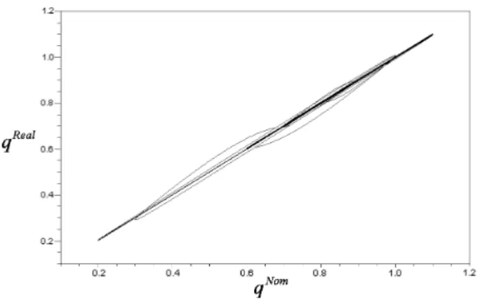
In case of no noise, Fig 4 illustrates the simulated phase space, while Fig 5 displays the connection between the nomi- nal and the realized trajectories. If the trajectories were exactly the same, Fig 5 would only contain one straight line. In Fig
Fig. 4. The simulated phase space without noise
Fig. 5. The connection between the nominal and the realized trajectories without noise
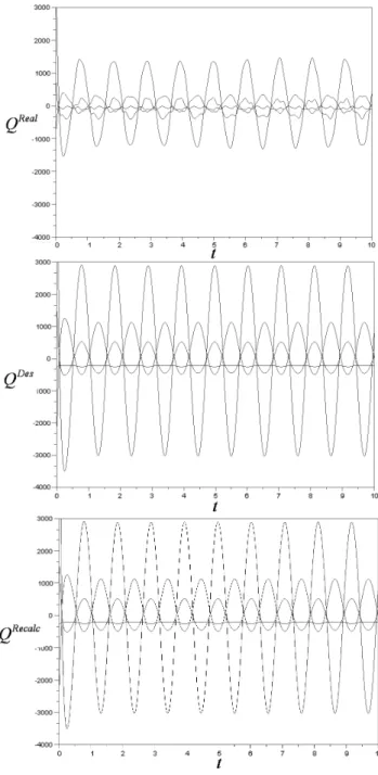
6 the realized, the desired and the recalculated torques are shown where the recalculation is made with the reference model and the real acceleration. Finally Fig 7 represents the tracking error.
In case of noise, Fig 8 displays the realized, the desired and the recalculated torques and Fig 9 illustrates the tracking error. In Fig 10 the connection between the nominal and the realized trajectories is shown. At the end, Fig 11 represents the simulated phase space.
VI. CONCLUSIONS
The difficulty of the solutions of many classical adaptive control problems with Lyapunov’s second or “direct” method led to focus on different approaches which are easier to use and are also advantageous concerned to the results. One of these methods is Robust Fixed Point Transformations which is based on Lyapunov’s Complete Stability theorem.
In this paper a novel approach is presented where an RFPT- based MRAC controller is suggested for poising two inverted pendulums on the top of a car. The car can move along a fixed horizontal line and the task is complicated with an extra hinge on one of the pendulums. The simulations show that the controller can manage and stabilize the system, and it is able to keep the pendulums in balance very well.
Fig. 6. The realized, the desired and the recalculated torque without noise
Fig. 7. The tracking error without noise
Fig. 8. The realized, the desired and the recalculated torque with noise
Fig. 9. The tracking error with noise
Fig. 11. The simulated phase space with noise
ACKNOWLEDGMENT
This work was sponsored by T ´AMOP 4.2.2./B-10/1-2010- 0020 and Applied Informatics Doctoral School at ´Obuda University in Hungary.
REFERENCES
[1] A.M. Lyapunov,A general task about the stability of motion(in Russian), PhD Thesis, 1892
[2] A.M. Lyapunov, Stability of motion, Academic Press, New-York and London, 1966
[3] Tanaka, K., Wang, H.O, Fuzzy Control Systems Design and Analysis.
New York: John Wiley & Sons, Inc., 2001
[4] V´arkonyi-K´oczy, A.R., State Dependant Anytime Control Methodology for Non-linear Systems, International Journal of Advanced Computational Intelligence and Intelligent Informatics (JACIII), Vol. 12, No. 2, pp. 198–
205, March 2008
[5] R. Isermann, K.H. Lachmann, and D. Matko,Adaptive Control Systems, Prentice-Hall, New York DC, USA, 1992
[6] Jean-Jacques E. Slotine, W. Li,Applied Nonlinear Control, Prentice Hall International, Inc., Englewood Cliffs, New Jersey 1991
[7] Charles C. Nguyen, Sami S. Antrazi, Zhen-Lei Zhou, Charles E. Campbell Jr.: Adaptive control of a stewart platform-based manipulator, Journal of Robotic Systems, Volume 10, Number 5, 1993, pp. 657–687
[8] R.M. Murray, Z. Li, S.S. Sastry: A mathematical introduction to robotic manipulation, CRC Press, New York, 1994.
[9] R. Kamnik, D. Matko and T. Bajd: Application of Model Reference Adaptive Control to Industrial Robot Impedance Control, Journal of Intelligent and Robotic Systems, vol. 22, pp. 153–163, 1998.
[16] J.K. Tar, I.J. Rudas and K.R. Kozłowski: Fixed Point Transformations- Based Approach in Adaptive Control of Smooth Systems. Lecture Notes in Control and Information Sciences 360 (Eds.: M. Thoma and M. Morari), Robot Motion and Control 2007 (Ed.: Krzysztof R. Kozłowski), Springer Verlag London Ltd., pp. 157–166, 2007.
[17] J.K. Tar, J.F. Bit´o, I.J. Rudas, K.R. Kozłowski, J.A. Tenreiro Machado:
Possible Adaptive Control by Tangent Hyperbolic Fixed Point Transforma- tions Used for Controlling theΦ6-Type Van der Pol Oscillator. In: Proc.
of the 6thIEEE International Conference on Computational Cybernetics (ICCC 2008), November 27–29, 2008, Star´a Lesn´a, Slovakia, pp. 15–20.
[18] J.K. Tar, J.F. Bit´o, L. N´adai, J.A. Tenreiro Machado: Robust Fixed Point Transformations in Adaptive Control Using Local Basin of Attraction, Acta Polytechnica Hungarica, Vol. 6 Issue No. 1, pp. 21–37, 2009.
[19] J.K. Tar, J.F. Bit´o, I.J. Rudas: Replacement of Lyapunov’s Direct Method in Model Reference Adaptive Control with Robust Fixed Point Transformations, Proc. of the 14th IEEE International Conference on Intelligent Engineering Systems 2010, Las Palmas of Gran Canaria, Spain, May 5–7, pp. 231–235, 2010.
[20] J.K. Tar, I.J. Rudas, J.F. Bit´o, K.R. Kozłowski, C. Pozna: A Novel Approach to the Model Reference Adaptive Control of MIMO Systems, Proc. of the 19th International Workshop on Robotics in Alpe-Adria- Danube Region (RAAD ’2010), June 23–25, 2010, Budapest, Hungary, pp. 31–36, (CD issue, file: 4 raad2010.pdf), 2010
[21] T.A. V´arkonyi, J.K. Tar, I.J. Rudas, Robust Fixed Point Transformations in Chaos Synchronization, Proc. of the 11th International Symposium on Computational Intelligence and Informatics (CINTI) 2010, Budapest, Hungary, 18–20 November, pp. 219–224, 2010
[22] T. Hovanyecz: “Comparative Study of Certain Nonlinear Control So- lutions” (in Hungarian), dissertation after a major study project, ´Obuda University, B´anki Don´at Faculty of Mechanical and Safaty Engineering, Budapest, Hungary, 2011
[23] Banach, S. “Sur les op´erations dans les ensembles abstraits et leur application aux ´equations int´egrales.” Fund. Math. 3, pp. 133-181, 1922 [24] Chung, C.C. and J. Hauser, “Nonlinear Control of a Swinging Pendu-
lum”, Automatica, Vol. 31, 1995
[25] K.H. Lundberg, J.K. Roberge: Classical dual-inverted-pendulum control, Proc. of 42ndIEEE Conference on Decision and Control, Vol. 5, pp. 4399- 4404, 2003
[26] Liu Li HE Hua-Can (School of Computer Science, Northwestern Poly- technical University, Xi’an 710072);Overview of the Stable Control of the Inverted Pendulum System[J];Computer Science;2006-05
[27] A. Bogdanov. Optimal control of a double inverted pendulum on a cart. Technical report CSE-04- 006, CSEE, OGI School of Science and Engineering, OHSU, 2004
[28] J.K. Tar, Towards Replacing Lyapunov’s “Direct” Method in Adaptive Control of Nonlinear Systems, (invited plenary lecture), Proc. of the 3rd Conference in Mathematical Methods in Engineering, 21–24 October 2010, Coimbra, Portugal, Paper 11 (CD issue) 2010
[29] J. Lam, “Control of an inverted pendulum,” http://www- ccec.ece.ucsb.edu/people/smith/student projects/Johnny Lam report 238.pdf