An opportunity of using Robust Fixed Point Transformation-based controller design in case of

An opportunity of using Robust Fixed Point Transformation-based controller design in case of

Type 1 Diabetes Mellitus

Levente Kov´acs^∗, Gy¨orgy Eigner^∗, Bence Czak´o^∗, M´at´e Siket^∗, J´ozsef K. Tar^†

∗Physiological Controls Research Center, Research, Innovation, and Service Center, Obuda University, Budapest, Hungary,´

Email: kovacs@uni-obuda.hu, eigner.gyorgy@nik.uni-obuda.hu, czako.bence@phd.uni-obuda.hu, siket.mate@gmail.com

†Antal Bejczy Center for Intelligent Robotics

Research, Innovation, and Service Center of ´Obuda University, Budapest, Hungary Email: tar.jozsef@nik.uni-obuda.hu

.

Abstract—In this paper a novel control strategy is introduced in order to create robust and adaptive control approach for type 1 diabetes mellitus. This approach uses Robust Fixed Point Transformations which hinders the negative effect of inherent model uncertainties and measurement disturbances. The results are validated by extensive simulation on the proposed control algorithm from which conclusions were drawn.

Index Terms—Robust Fixed Point Transformation, Nonlinear Control, Cyber-medical Systems

I. INTRODUCTION

Modeling and control of biological systems is a difficult task in which the classical mathematical tools mostly inap- plicable because of several unfavourable properties of such systems e.g. non-linear behaviour, often occurring saturations, and time-delays. In the recent years in-silico modeling and testing became extremely important due to the advancement of computational methods and the decreasing numbers of in-vivo laboratory experiments on living organisms. When the task is to develop approximate models of physiological systems concerning human beings and to use these models in controller design in order to handle some properties of living organisms, the effects of modeling imprecisions become more and more critical [1]. The aforementioned effects typically occur in the control of Diabetes Mellitus (DM). While DM is an incurable disease, the treatment of the metabolic system is possible concerning insulin hormone. Insulin is produced by pancreatic β-cells and plays a crucial role in dispensing the main energy source - glucose - through the cell-wall of adipose tissues and striated muscle cells with insulin-regulated glucose trans- porters, regulating (with other hormones) the glycogenesis- glycogenolysis cycle and other important processes [2]. From

B. Czak´o was supported by the ´UNKP-18-3. New National Excellence Program of the Ministry of Human Capacities. This project has received funding from the European Research Council (ERC) under the European Union’s Horizon 2020 research and innovation programme (grant agreement No 679681)

all the types of DM the most dangerous is Type 1 DM (T1DM) which is associated with the lack of insulin caused by the destruction of β-cells during an autoimmune reaction [3].

In the case of T1DM the patient requests external insulin administration in order to maintain its glycemia. In general the treatment can be done manually by the use of an insulin pen or can be automated by insulin pumps [3] however regardless of the administration methodology the main goals of such ther- apies are the same: avoidance of hypoglycemia, moderately occurring hyperglycemia [4] and/or low variability of glycemia [5]. From an engineering point of view, the insulin pump based Artificial Pancreas (AP) concept might be the best solution in order to reach the optimal glycemia. The AP concept is based on Continuous Glucose Monitoring Sensors (CGMS) [6], an insulin pump, and advanced control algorithms [8]. In this study we investigate the applicability of the recently developed RFPT-based control design methodology for T1DM control.

The developed algorithms are able to deal with the different glycemic loads caused by daily nutrition.

The paper is structured as follows: the RFPT methodology and design steps are introduced first followed by a case study concerning the operation of the controller, on which conclusions are drawn with a discussion of future research directions.

II. RFPT-BASED CONTROLLER DESIGN IN CASE OF PHYSIOLOGICAL PROCESSES

The RFPT methodology can be introduced by the realized- response scheme as described in [9], [10]. The underlying idea is that upon inverting the model of the system, one can obtain a proper control signal which steers the controlled states along a desired trajectory. The profound issue is that in almost every case the parameters of the inverted model are not exactly the same in relation to the exact model so that the calculated input will cause a different behaviour of the physical system. The RFPT tackles this issue by deforming the desired trajectory in a way that the physical system will behave as one would

978-1-7281-3345-4/19/$31.00 c2019 European Union

require. This can be achieved by using a deform function which in SISO case is defined as follows according to [9], [11]:

r_n+1=G(r_n;r^Des),(r_n+K_c)×

1 +B_c

tanh(A_c(f(r_n)−r^Des)) −K_c , (1) where K_c, A_c, and B_c = ±1 are the control parameters.

The function has to be iterated as {r0

def= r^Des, r1 = G(r0). . . , rn+1 = G(rn), . . .} so that a proper fixed point can be achieved. A detailed description of the operation and the structure of the controller can be found in [9] and [11].

A detailed description of the controller design procedure is described next, beginning with the general properties of the mathematical model of the phenomenon that we wish to use in the control. By revealing the more specific model properties an effect chain can be deduced that determines the relative order of the control task. Using a simple approximate model the need for the information on the components of certain state variables can be evaded. The adaptivity of the designed controller can compensate for the effects of these modeling imprecisions.

A. Modeling difficulties in general

In diabetes research mathematical modeling of the physio- logical processes and the in-vitro investigations have impor- tant relevance due to the fact that the possibility of in-vivo experiments are limited since the subjects of the examinations are human beings. In such investigations the real patients are substituted with models of various complexity called patient models, which can be completed with other sub-models (e.g.:

absorption model, sensor model, noise model, etc.) in order to simulate the behaviour of the human metabolic system regarding the glucose-insulin household. However when the available mathematical models are utilised during the con- troller design, several unfavourable model properties might appear such as strong non-linearities and time delay effects that are essential parts of the reality [1]. Efficient handling of the intra- and inter-patient variability is also a challenging aspect, since a virtual patient can be described with a given parameter set of the mathematical model. Furthermore an identified individualized virtual patient model belongs only to the patient under consideration so that the model can not be used in general terms. That means that the model-based controller design solutions based on a virtual patient model as exact model may be seriously affected by these problems:

they can handle only a particular group of patients who have the same metabolic attitudes. However in spite of these unfavourable circumstances, maintaining the generality of the controller and in the same time providing personalized control would be most beneficial. In general adaptive controllers could provide such solutions. Specifically the RFPT-based adaptive controller design methodology could be a possible candidate due to that fact that it requires only a roughly approximate mathematical model of the controlled phenomenon.

B. Investigation of the effect chain of the control action In order to realize the RFPT-based controller an inverse model must be established which effectively captures the approximate dynamics of the connection between the control signal (the injected insulin) and the controlled variable (the Blood Glucose (BG) level). The most simple way is using a virtual patient model at this point instead of a real patient, however models can be created based on measurements as well. Three possible cases can occur:

• Real patient data is used: a model can be created that describes the relationship between the insulin signal and the BG level;

• Simple virtual patient model is used: usually, the insulin affects higher derivatives of the BG level via simple interconnections that determine the necessary order of the control law; the model structure can be considered and transformed to an approximate model to capture this dynamics;

• Complex virtual patient model is used: insulin affects high derivatives of the BG level via complex intercon- nections; the model structure cannot be used during the approximate model design.

C. Designing the approximate model

If BG measurements and insulin injection data are available of the real patient, a general mathematical model can be created and the well known identification procedures also can be employed at this point. The main restrictions are that the carbohydrate (CHO) intake can be considered only as a random disturbance input and in the case when insulin injec- tions are known the CHO intake still has an impulse attitude.

Moreover the sensor noise influences the BG measurements.

Beside these unfavourable circumstances the goal is to create such a mathematical model, which can approximately catch the dynamics of the process. For example, a nonlinear discrete autoregressive-type NARMAX model can be a reasonable choice because of its simplicity and general applicability [12].

The rough approximation model can be also generated from the given patient model if its structure is simple which is true in the presence of only a few state variables. This does not correspond to model-based process in the classical sense, although the model structure is utilized during the procedure.

The parameters of the model can be arbitrarily determined or randomized within reasonable limits. For instance, assume that the original first order non-linear system is described as

G(t) =˙ f(t, G(t), u(t), d(t)) . (2) where variableGdenotes the BG level. Via restructuring the equation, the dynamic connection among the insulin input and the first derivative of the BG level will be:

u(t) =h(t,G(t), G(t), u(t), d(t))˙ . (3) In the case of more complex models it can happen that the in- sulin input influences directly the higher order derivative of the

BG level. If the insulin input modifies directly only a very high order derivative ofGthe use of this model in its original form is not sufficient. Although certain parts of the original models can be considered during the approximate model design, (e.g.

the connections between the subsystems), the complex model can be handled as a virtual patient and similar techniques can be used as in the first case when the patient measurements are available. That means that measurements can be generated based on in-silico trials and identification can be applied.

However a different approach exists as well. Since the macro- scaled physiological processes are slowly varying the Quasi Stationary Theorem (QST) from classical thermodynamics [13] can be used in approximate model design. The principle of the approach is that the inputs can be mapped by little modification of the stationary outputs if the solution of the equations of motion is stable stationary for stationary inputs.

D. Selection of the control law

Since the design of the RFPT-based adaptive controller is commenced with the determination of a purely kinematic prescription of the tracking error, a proper function has to be elaborated. While various possibilities can be employed, in many cases (and this in particular) a PID type tracking can be considered which is defined as:

d dt+ Λ

⁽ⁿ⁺¹⁾Z^t

t₀

G^N(ξ)−G(ξ)

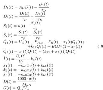
dξ= 0, (4) where n is the relative degree of the system, Λ is a control parameter, G^N(t) is the desired BG concentration to be tracked, G(t)is the realized BG concentration, and the error signal is the e(t) =G^N(t)−G(t)ought to converge to zero in infinity, i.e. e → 0 as t → ∞. On the subject of the aforementioned considerations a general RFPT-based T1DM control environment can be finalized as it is shown in Fig. 1.

It also depends on the approximate model to be applied.

E. Considerations and restrictions regarding the controller design in case of T1DM

Modeling and control of T1DM is effected by several unfavourable practical and physiological constraints. These could be the lack of information on the internal state variables of the patient model (as it is in the case of a real patient), the impulse nature of the inputs, the output (the BG level) being quantized and not available in every time instant, the controller cannot administer arbitrarily big insulin ingress for example.

Every mentioned impacts can be handled with sub-models or restrictions that increase the complexity of the model.

Naturally, simplifications can be done in order to reduce the complexity. During our investigations we applied simplifica- tions in modeling the feed intake. Since the absorption sub- models well characterise the rate of glucose appearance in the blood generally (they provide satisfying approximations), it is assumed that the outputs of the applied absorption models are known. Furthermore, the total amount of insulin consumed in

Figure 1. General structure of a RFPT-based controller: the two delay blocks correspond to the cycle time of the digital controller

the control of glycemia is also important: practically this value is limited.

III. CONTROL OF THEHOVORKA MODEL

In order to demonstrate and prove the usability of the RFPT- based design methodology, the Hovorka T1DM model was selected which is frequently used among scientific researches [14], [15]. Instead of applying parameter identification, mod- els with their given parameters were chosen so that further comparison could be done in the literature. Since the primary goal was the introduction of a new controller design method this was a reasonable choice. During our investigations adverse circumstances were applied, namely high glucose amounts and long simulation time, in order to prove the long term usability of the developed controllers.

A significant difficulty should be noted regarding the use of PID type laws. Since the controller can only decrease the BG level with the control signal and the feed intake is a disturbance from this point of view dead periods may occur in the control after the insulin injections. If too much insulin is injected, which may causes dangerous decrease in the BG level, the controller has to wait for the depletion of the insulin via the natural channels because there is no practical means to extract insulin from the human body. (The desired control action in this case should cause instant decrease in the insulin level that is impossible. The best realizable control signal in this case is the zero insulin ingress rate.) Furthermore the integrated error could considerably increase during the dead periods. There are several solutions to this problem, namely the application of other (e.g. PD-type) control laws, or cutting the error signal at zero if the prescribed nominal BG level G^N is higher than the actual G(t). In this case the PID type control law was appropriate without modification.

The model under investigation was the Hovorka model described by (18), which is a complex T1DM model. It originally occurred in [16], but in this study a slightly different model was used from [17]. Due to the lack of space the the state variables are not detailed here but can be found in [16], [17]. The model has ten state variables that describe not just only the glucose-insulin dynamics but also captures the externally injected insulin’s absorption and distribution, the insulin effects, the insulin independent BG changes, and the internal glucose production too. Moreover it also contains an embedded glucose absorption model. The model equations in conjunction with the description of the parameters can be found in the Appendix.

The relative order of the possible kinematic control type is five since the input signal appears in the 5th derivative of the controlled state Q1(t). This entails that high order derivative is presented from (18) in the approximate model. Because of the relative order, the 5th derivative of the controlled state Q₁(t) must be determined. The relative order implies that some simplification should be imposed on the exact model.

Two different types of simplifications can be utilized: the use of parameter approximation instead of exact parameters or neglecting parts from the model elements. Both of these restrictions were applied on the approximate model.

The 5th order derivative of Q1(t)was carried out first, which can be derived from (18):

Q⁽⁵⁾₁ (t) =D⁽⁴⁾₂ (t) VGτD

−F_01,c⁽⁴⁾ −F_R⁽⁴⁾

−x⁽⁴⁾₁ (t)Q1(t)−4x⁽³⁾₁ (t) ˙Q1(t)− −5¨x1(t) ¨Q1(t)−

4 ˙x1(t)Q⁽³⁾₁ (t)x1(t)Q⁽⁴⁾₁ (t) +k12Q⁽⁴⁾₂ −EGP0x⁽⁴⁾₃ (t) .

(5) Equation (5) can be rearranged and completed with a new term, the affine parameterA, which represents each neglected elements. Thus the control signal directly appears in x⁽⁴⁾₁ (t) and x⁽⁴⁾₃ (t) state derivatives, hence the approximate model takes the form of:

Q⁽⁵⁾₁ (t) =−x⁽⁴⁾₁ (t)Q₁(t)−EGP₀x⁽⁴⁾₃ (t) +A . (6) The 4th order derivative of x⁽⁴⁾₁ (t) and x⁽⁴⁾₃ (t) can be derived from the model equation (18), however the presence of the control signal has to be identified first. This can be done by using the following equations:

S˙1(t) =u(t)−S1(t)

τ_S . (7)

S¨₂(t) = S˙1(t)

τS

− S˙2(t)

τS

=u(t) τS

−S1(t) τ_S² −

S˙2(t) τS

. (8)

I⁽³⁾(t) = S¨2(t)

V_Iτ_S −keI(t) =¨ u(t)

V_Iτ_S²−S1(t) V_Iτ_S³−

S˙2(t)

V_Iτ_S²−keI(t)¨ . (9)

x⁽⁴⁾₁ (t) =−ka1x⁽³⁾₁ (t) +kb1I⁽³⁾(t) =

=−ka1x⁽³⁾₁ (t) +kb1

u(t)

VIτ_S²−S1(t) VIτ_S³−

S˙2(t)

VIτ_S²−keI(t)¨ .

(10)

x⁽⁴⁾₃ (t) =−ka3x⁽³⁾₁ (t) +k_b3I⁽³⁾(t) =

=−ka3x⁽³⁾₃ (t) +kb3

u(t)

VIτ_S²−S1(t) VIτ_S³−

S˙2(t)

VIτ_S²−keI(t)¨ .

(11) Equation (10) and (11) can be substituted into (6). More- over, the neglected subparts can be incorporated in variableA as follows:

Q⁽⁵⁾₁ (t) =−k_b1u(t)

V_Iτ_S²Q₁(t)−EGP₀k_b3u(t)

V_Iτ_S²+A . (12) From (12), one can rearrange the equation so that the connection between the control signal and the 5th derivative of Q₁(t)leads to:

u(t) = Q⁽⁵⁾₁ (t)−A

−k_b1Q₁(t)−EGP₀k_b3VIτ_S² =

= −Q⁽⁵⁾₁ (t) +A kb1Q1(t) +EGP0kb3

VIτ_S²

. (13)

Equation (13) is a proper candidate for an approximate model. We applied further modifications since the exact model parameters are not available in every case. The finalized approximate model that we utilized in this study was the following:

u(t)≈ −Q⁽⁵⁾₁ (t) +Aconst

k_b1appQ₁(t) +EGP_0appk_b3appVI_appτ_S²

app , (14) where a 10% random deviation was used in the approx- imated parameters. Moreover the affine A parameter was replaced with a constant Aconst.

For the kinematic part of the controller a simple PID type prescription was employed. One can assume that the glucose distribution volume is known at this point as well which allows writing the kinematic type PID control law to Q₁(t) in the form of:

Q^(5),Des₁ (t) =Q^(5),N₁ +

5

X

s=0

6 s

Λ^6−s d

dt ^s

·

·

t

Z

t₀

Q^N₁ (ξ)−Q1(ξ) dξ

(15)

IV. SIMULATION RESULTS

In the current simulation realistic circumstances were in- troduced to the highest extent possible. For this purpose practical feed intake protocol were employed based on the recommendations of the World Health Organization (WHO) [18]. In order to apply this protocol the treatment assumed a 27years old female patient of70kgweight with little physical activity. Based on the WHO recommendations the required calorie intake for a day is described by (16) [18]:

CHO_req/day = 15.3BW+ 679 = 1750kcal

day . (16) Since the applied absorption model contains the CHO as the only input parameter an assumption was made that the total calorie intake was made up from only CHO, namely glucose. Generally speaking the carbohydrates and complex meals have lower glycemic index and needs longer absorption, therefore this simplification can be considered as a worst case scenario, because of the fast increment of the glucose concentration in the blood. Since accurate coordination of the feed intakes cannot be provided (it depends on the lifestyle) a randomization was designed in the amounts and time frames of the glucose intakes. Furthermore1gCHO is equivalent with 4.2kcal [4] the total calculated CHO intake should be equal with416.667g. The amount was divided into five parts; three bigger meals (breakfast, lunch, dinner) and two smaller meals (snacks). Randomization were made in the amounts and time frames of different intakes as can be seen in Table I. Moreover

Table I

RANDOMIZATION OF THE GLUCOSE INTAKES

Notation Amount[g] Duration [min]

Time of intake [min]

CHObreakf ast

20−25%of

CHOreq/day 15±5% 210±5%

CHOsnack1

10−15%of

CHO_req/day 10±5% 390±5%

CHO_lunch 25−30%of

CHO_req/day 20±5% 510±5%

CHOsnack2

10−15%of

CHOreq/day 10±5% 780±5%

CHOdinner

20−25%of

CHO_req/day 20±5% 900±5%

a strict constraint was applied on the total calorie intake in the form of:

CHObreakf ast+CHOlunch+CHOdinner=

= 75% of CHO_req/day CHO_snack1+CHO_snack2= 25% of CHO_req/day

. (17)

The simulations were made in Scilab^TM and the figure plots were created with M AT LAB^TM. The initial states of the 48 hours long simulation were xini(t) = [D1,ini, D2,ini, S1,ini, S2,ini, Iini, x1,ini

, x2,ini, x3,ini, Q1,ini, Q2,ini]^T = [0,0,687.5,687.5,10.783,5.521e−2,8.842e−3,0.5607e−

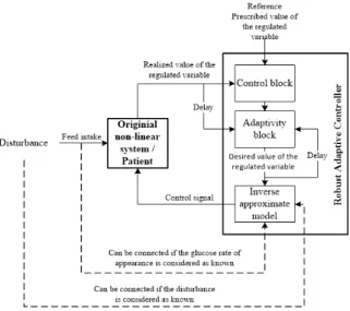
1,86.3,63.66]^>. The results of the numerical simulations are presented in Fig. 2. Without external glucose intake the BG level is increasing due to the glucose secretion of the liver which is embedded in the model. The applied controller starts the insulin injection when the BG level is increasing and turns off upon decreasing BG level. This switching attitude can be derived from the applied control strategy and this is a consequence that the controller cannot apply negative control input. It can be seen that despite of the continuously absorbing external glucose concentration the controller can manage the glycemia and able to avoid the hypoglycemia while minimizing the hyperglycemia. The latter cannot be totally eliminated because of the high and random glucose intakes. On the basis of the numerical results it can be stated that the controller could achieve its goal and operated as expected.

Time [min]

0 500 1000 1500 2000 2500

BGlevel[mmol/L]

5 10 15

Blood glucose level

Time [min]

0 500 1000 1500 2000 2500

Insulin [mU]

0 50 100

150 Injected insulin

Time [min]

0 500 1000 1500 2000 2500

Absorbedglucose[mmol/L]

0 5

10 Blood glucose level

Figure 2. Results of the 48 hours long simulation of the Hovorka model [Q^N₁ = 90mmol/L (G^N =Q^N₁ /VG ≈8.036mmol/L),Λ = 1e−4, Ac= 1/10|K_c|,Kc= 5e−1andBc=−1]

V. CONCLUSION

In this paper, our goal was to provide a general overview about the RFPT-based controller design approach. While these solutions can be extended into other physiological areas, we focused to the control of T1DM in our research. We showed the full path of the RFPT-based controller design in case of physiological systems step-by-step. Moreover we demonstrated the design approach in case of T1DM control via case studies. The RFPT-based control design approach has several benefits against model-based control design; these advantages were detailed in the text. However, in this study we did not apply parameter optimization on the controller

parameters, or identification on the used T1DM models which we are going to investigate in our future work.

REFERENCES

[1] J. Bronzino and D. Peterson, The Biomedical Engineering Handbook, 4th ed. Boca Raton, Florida, USA: CRC Press, 2015.

[2] D. R. Ferrier, Biochemistry, 6th ed. Baltimore, Maryland, USA:

Lippincott Williams and Wilkins, 2014.

[3] International Diabetes Federation,IDF Diabetes Atlas, 8th ed. Brussel, Belgium: International Diabetes Federation, 2017.

[4] R. DeFronzo, E. Ferrannini, P. Zimmet, and G. Alberti, Eds.,Interna- tional Textbook of Diabetes Mellitus, 4th ed. New Jersey, US: Wiley- Blackwell, 2015.

[5] T. Ferenci, A. K¨orner, and L. Kov´acs, “The interrelationship of hba1c and real-time continuous glucose monitoring in children with type 1 diabetes,”Diabetes Res Clin Pr, vol. 108, no. 1, pp. 38–44, 2015.

[6] Zavitsanou, S. and Lee, J.B. and Pinsker, J.E. and Church, M.M. and Doyle III, F.J. and Dassau, E., “A personalized week-to-week updating algorithm to improve continuous glucose monitoring performance,”

Journal of diabetes science and technology, vol. 11, no. 6, pp. 1070–

1079, 2017.

[7] D. Copot, R. De Keyser, J. Juchem, and C. Ionescu, “Fractional order impedance model to estimate glucose concentration: in vitro analysis,”

ACTA Pol Hung, vol. 14, no. 1, pp. 207–220, 2017.

[8] F. Chee and T. Fernando, Closed-Loop Control of Blood Glucose.

Heidelberg, Germany: Springer, 2007.

[9] J.K. Tar, J.F. Bit´o, L. N´adai, and J.A.T. Machado, “Robust fixed point transformations in adaptive control using local basin of attraction,”ACTA Pol Hung, vol. 6, no. 1, pp. 21–37, 2009.

[10] L. Kov´acs, “A robust fixed point transformation-based approach for type 1 diabetes control,”Nonlinear Dynamics, vol. 89, no. 4, pp. 2481–2493, 2017.

[11] J. K. Tar, L. N´adai, and I. J. Rudas,System and Control Theory with Especial Emphasis on Nonlinear Systems. Typotex, 2012.

[12] S.A. Billings,Nonlinear System Identification, 1st ed. Chichester, UK:

John Wiley & Sons, 2013.

[13] D. Kondepudi and I. Prigogine,Modern Thermodynamics: From Heat Engines to Dissipative Structures, 2nd ed. Chichester, UK: John Wiley

& Sons, 2014.

[14] P. Palumbo, S. Ditlevsen, A. Bertuzzi, and A. de Gaetano, “Mathematical modeling of the glucose–insulin system: A review,”Math Biosci, vol.

244, pp. 69 – 81, 2013.

[15] V.N. Shah, A. Shoskes, B. Tawfik, and S.K. Garg, “Closed-loop system in the management of diabetes: Past, present, and future,” Diabetes Technol The, vol. 16, no. 8, pp. 477–490, 2014.

[16] R. Hovorka, F. Shojaee-Moradie, P.V. Carroll, L.J. Chassin, I.J. Gowrie, N.C. Jackson, R.S. Tudor, M. Umpleby, and D.H. Jones, “Partitioning glucose distribution/transport, disposal, and endogenous production dur- ing IVGTT,”Am J Physiol Endocrinol Metab, vol. 282, no. 5, pp. E992 – 1007, 2002.

[17] M. Naerum, “Model predictive control for insulin administration in people with type 1 diabetes,” Technical University of Denmark, Tech.

Rep., 2010.

[18] K.P. Sucher, M. Nelms, S. Long-Roth, and K. Lacey,Nutrition Therapy and Pathophysiology. Cengage Learning, 2011.

APPENDIX

The equations of the Hovorka model are the following [16], [17]:

D˙1(t) =AGD(t)−D1(t) τD

D˙2(t) =D1(t) τD

−D2(t) τD

S˙1(t) =u(t)−S1(t) τS

S˙2(t) =S1(t) τS

−S2(t) τS

Q˙1(t) =UG(t)−F01,c−FR(t)−x1(t)Q1(t)+

+k12Q2(t) +EGP0(1−x3(t)) Q˙2(t) =x1(t)Q1(t)−(k12+x2(t))Q2(t) I(t) =˙ UI(t)

VI

−keI(t)

˙

x1(t) =−ka1x1(t) +kb1I(t)

˙

x2(t) =−ka2x2(t) +kb2I(t)

˙

x3(t) =−ka3x3(t) +kb3I(t) D(t) = 1000·d(t)

MwG

G(t) =Q1/VG

(18)

The following table contains the parameters, their descriptions and their values which were used in this study regarding the Hovorka model [16], [17]:

Table II

PARAMETERS AND THEIR DETAILS IN THE USEDHOVORKA MODEL

Notation Unit Description Value

BW kg Body weight 70

MwG g/mol Molecular weight of glucose

180.15588

k12 min⁻¹ Transfer rate 0.066

ka1 min⁻¹ Deactivation rate 0.006

ka2 min⁻¹ Deactivation rate 0.06

ka3 min⁻¹ Deactivation rate 0.03

ke min⁻¹ Insulin

elimination rate

0.138

τD min CHO absorption

constant

40

τS min Insulin

absorption constant

55

AG − CHO to glucose

utilization

0.8

VI/BW L·kg⁻¹ Insulin distribu- tion volume

0.12

VG/BW L·kg⁻¹ Glucose distribu- tion volume

0.16

EGP0/BW L·kg⁻¹min⁻¹ Liver glucose production at zero insulin

0.0161

F01/BW L·kg⁻¹min⁻¹ Insulin indepen- dent CNS con- sumption

0.00097

S_IT L/mU Insulin sensitivity

of transport / dis- tribution

51.2·10⁻⁴

SID L/mU Insulin sensitivity

of disposal

8.2·10⁻⁴

SIE L/mU Insulin sensitivity

of EGP

520·10⁻⁴