Óbuda University

(1)

Óbuda University

Generalization of Tensor Product Model Based Control Analysis and Synthesis

Ph.D. Theses

József Kuti

Supervisor:

Dr. Péter Galambos

Budapest 2018

(2)

Szigorlati bizottság:

Prof. Dr. Tar József Kázmér: Rendszer és irányításelmélet Prof. Dr. Szalay Tibor: Robotika

Prof. Dr. Galántai Aurél: Mátrixanalízis

Házivédés oppenesek:

Prof. Dr. Huijun Gao (Harbin Institute of Technology) Dr. Drexler Dániel (Óbudai Egyetem)

Nyilvános védés opponensek:

Dr. Takarics Béla (MTA SZTAKI) Dr. Kovács Levente (Óbudai Egyetem)

(3)

Acknowledgments

I am grateful to my supervisor, Dr. Péter Galambos, who introduced me to the world of research during our collaboration since 2012. This thesis was motivated by his practical, straightforward attitude and by the inspiring atmosphere of scientific research and development he established.

I also wish to thank Prof. Péter Baranyi, who gave me the opportunity to follow my thoughts during the three years I spent in MTA SZTAKI.

I would like to thank my former colleagues, Prof. Zoltan Szabó, Prof. Gyula Sallai, Dr. Ádám Csapó and Dr. Béla Takarics for all the help I received from them.

I would also like to express my appreciation to Doctoral School of Applied Informatics and Applied Mathematics of Óbuda University and Research and Innovation Center of Óbuda University and teachers of Budapest University of Technology and Economics, who highly motivated me during that years: Prof. Gábor Stépán who showed the nature of dynamical systems and gave analytical tools to investigate it, Prof. Antal Huba who presented the role of engineers to influence their behaviour, and finally Prof. József Bokor and Prof. Béla Lantos who allowed me to learn about the essence of control theory.

Last, but not least, special thanks to my parents and my family, who have supported me during the whole period of my studies.

The research was supported by the Hungarian National Development Agency, (ERC- HU-09-1-2009-0004 MTASZTAK) (OMFB-01677/2009), by the Hungarian State and the European Union under the EFOP-3.6.1-16-2016-00010 project and by the UNKP- 16-3 New National Excellence Program of the Ministry of Human Capacities.

(4)

Declaration

Undersigned, József Kuti, hereby state that this Ph.D. Thesis is my own work, wherein I only used the sources listed in the bibliography. All parts taken from other works, either as word for word citation or rewritten keeping the original meaning, have been unambiguously marked, and reference to the source was included.

Nyilatkozat

Alulírott Kuti József kijelentem, hogy ezt a doktori értekezést önállóan készítettem, és abban csak a listában szereplő forrásokat használtam fel. Minden olyan részt, amelyet szó szerint szerint, vagy azonos tartalomban, de átfogalmazva más forrásból átvettem, egyértelműen a forrás megadásával megjelöltem.

Budapest, April 20, 2018

József Kuti

(5)

List of Figures

3.1 Illustrations for tensor operations . . . 19

3.2 TP model transformation (N=2) . . . 24

3.3 The new control design workflow and the role of the chapters . . . 30

4.1 Illustration of the used notations: the considered function c:𝑋 →𝐻, the affine hull A of the image set, that is here 𝐷 = 2 dimensional, orthogonal basis (a₁,a₂), offset to it a₃, the convex hull of the image setC, enclosing polytope with vertices (s₁,s₂,s₃). . . 32

4.2 Illustration of unique weighting functions of simplex polytopic forms . 39 5.1 Illustrations of extended tensor operations . . . 44

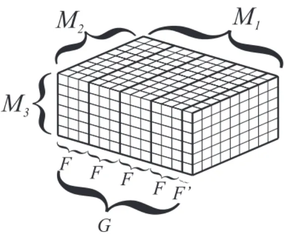
5.2 Illustration of discretisation using piecewise linear interpolatory functions 51 5.3 Illustration of partitions if 𝐾 = 3, 𝑀₁ = 13, 𝑀₂ = 9, 𝑀₃ = 6, 𝐹 = 3, 𝐹^′ = 1, 𝐺= 5 . . . 54

5.4 Illustration of Algorithm 5.20 considering the case depicted in Fig. 5.3 56 6.1 Enclosing polytope as intersection of halfspaces (given by n_𝑖 normals and 𝛼𝑖 offsets) . . . 76

8.1 Inverted pendulum model . . . 91

8.2 The weighting functions of the Affine TP model . . . 96

8.3 The weighting functions of the Affine TP model via discretisation . . 96

8.4 The weighting functions of the MVS polytopic TP model . . . 98

8.5 Minimal volume enclosing simplex for v⁽¹⁾(𝑝₁)function . . . 99

8.6 The results of controller design (A) . . . 100

8.7 The results of controller design (B) . . . 101

8.8 The results of controller design (C) . . . 102

8.9 The achievable 𝛾∞ disturbance rejection with different variable com- plexities . . . 103

8.10 Minimal volume enclosing simplex for v⁽¹⁾(𝑝1)function . . . 104

(9)

8.11 Minimal volume enclosing simplex for v⁽¹⁾(𝑝₁)function . . . 105 9.1 Mechanical model of the vibrating system . . . 107 9.2 Simulation results: Three short vibration impulses show that the fre-

quency and amplitude are adjustable independently. . . 108 9.3 The mechanical model of the TORA system . . . 109 9.4 The results of optimisation LMI on manipulated models, the dash line

shows the minimal feasible 𝜈 value for all S(p) system matrices for comparison . . . 110 9.5 The MVS enclosing polytope and the cut one . . . 111 9.6 Behaviour of the controlled system . . . 111 10.1 The new control design workflow and role of the elaborated theses . . 113 10.2 Illustration of discretisation via multivariate interpolatory functions . 115 A.1 Illustration of SNNN enclosing polytope generation . . . 120 A.2 Illustration of A, B, C, D steps for a given 𝛼 . . . 122 A.3 Phases of CNO enclosing polytope generation for a𝐷= 2problem and

given 𝜙₁, 𝜙₂, 𝜙₃ values . . . 123

(10)

Preface

During my master’s diploma research and period of the Young Research Award, I have applied the TP model transformation and basic LMI-based control design methods to different non-linear and time-delay feedback problems:

1. A haptic telemanipulator arm with time-delayed communication and unknown remote environment, where the effect of time-delay must be decreased because it influences the sensed properties of the remote environment and may cause unstable behavior.

2. The prototype of the so-called dual-excenter actuator. That is a special vibration actuator that is able to work at independently chosen frequency and amplitude in contrast to the widely used vibration devices. Its control is chal- lenging because of its highly non-linear behavior and the unknown working environment.

The development and the corresponding theoretical and numerical supervisions dredged up more practical demand and sources of conservativeness. These experiences motivated my Ph.D. research to extend and renew the theoretical basis of TP model transformation based controller design.

The dissertation

– introduces new concepts and numerical methods to deal with practical chal- lenges of modeling and control design,

– deeply renews the abstract, mathematical formalism of Tensor-Product Model- based control analysis, synthesis and the corresponding transformation method.

For the sake of generality, the elaborated definitions are characterized in an abstract mathematical way, and the corresponding proofs are provided as well. Similarly, the proposed numerical methods were described for general cases - that cover usually higher dimensional geometry, tensors with arbitrary number of dimensions, models that depend on arbitrary number of parameters, that are given in arbitrary number of parameter sets – that is necessary to see the nature of problems and the proposed methods to handle them.

(11)

Goals of the thesis

Tensor product models are multi-polytopic forms of Linear Parameter Varying (LPV) and quasi-LPV (qLPV) models separating their parameter dependencies. The motivation of their application is the existence of “automatic” numerical methods to obtain this kind of polytopic models and the numerous control analysis and synthesis methods that can be immediately applied to them.

The theses of this dissertation extend the practical opportunities and revise the methodology by taking into account the current problems:

1. In many cases, the infeasibility of controller synthesis was apparently caused by the actual structure of polytopic TP model, but there was no method that can efficiently, fast and repeatably generates and fine manipulate the polytopic structures. Furthermore, the existing methods are only capable of providing simplex polytopes.

2. Although the Higher Order Singular Value Decomposition (HOSVD) based Ten- sor Product form gives a good description about algebraic structure and complexity of the model, it is not really connected to the problem of generating a polytopic form. The nature of these problems is geometric, and the intermedi- ate state is expected to represent the affine geometric structure of the model, which, however, is not provided by the former HOSVD based approach.

3. The separation of the parameter dependencies into a multi-polytopic structure may increase the complexity but was not exploited during controller design.

There is a practical need either for lossless polytopic models for some cases and for a controller design approach that can exploit the parameter separations by handling them in different ways (according to their practical properties).

For example, to apply controller candidates that depend only on the measur- able parameters, and Lyapunov-candidates that depend only on the constant parameters, etc.

(12)

Structure of the dissertation

The dissertation is structured as follows:

The first part of the dissertation describes the related basic concepts.

∙ Chapter 1 gives a brief review of the history of control theory, clarifying the motivation of robust and optimal control design, and highlighting the relevance of Lyapunov’s works.

∙ Chapter 2 details the LPV/qLPV modeling, its relationship to the LMI based controller design and the importance of convexity.

∙ Following that, Chapter 3 presents the concept of TP Model Transformation as the main objective of the theoretical research.

The second part of the dissertation presents the theoretical achievements.

∙ Chapter 4 shows the role of affine descriptions to derive polytopic forms and proposes the unique ASVD for this purpose.

∙ Chapter 5 generalizes the result to derive polytopic TP forms and proposes further extensions of the definitions.

∙ After that, Chapter 6 considers the geometric problem to generate and manipulate enclosing polytopes according to the control goals.

∙ Finally, Chapter 7 describes the extended concept of Polytopic TP model-based control analysis and synthesis, which generalizes the polytopic TP model-based controller design.

The third part shows the application of the proposed concepts and methods on practical problems.

∙ Chapter 8 provides a detailed numerical example by considering the simple 2D inverted pendulum problem.

∙ Chapter 9 summarizes the achieved results on the dual-excenter vibrotactor and the translational oscillator with rotational actuator (TORA) systems.

The fourth part concludes the scientific results in five theses.

(13)

Nomenclature

The following abbreviations and notations are used along the dissertation:

LTI Linear Time Invariant

(q)LPV (quasi)Linear Parameter Varying

LQR, LQG Linear Quadratic Regulator, Linear Quadratic Gaussian LMI Linear Matrix Inequality

SDP Semidefinite Programming

SQP Sequential Quadratic Programming

SOS Sum of Squares

SVD Singular Value Decomposition

ASVD Affine Singular Value Decomposition

HOSVD Higher Order Singular Value Decomposition HOOI Higher Order Orthogonal Iteration

TP model Tensor Product model

MVS, MVSA Minimal Volume Simplex, Minimal Volume Simplex Analysis PDC Parallel Distributed Compensation

For scalars:

𝑎, 𝑏, . . . scalar values

𝛿𝑖𝑗 Dirac-delta (𝛿𝑖𝑖= 1, 𝛿𝑖𝑗 = 0 if 𝑖̸=𝑗) 𝑥, 𝑥 lower and upper bounds for the 𝑥 scalar

For vectors and matrices:

a,b, . . . vectors A,B, . . . matrices

0^𝑎×𝑏,1^𝑎×𝑏 𝑎×𝑏 size matrix of zeros/ones E^𝑎×𝑏 𝑎×𝑏 size identity matrix

M^𝑇 transposed matrix

Sym(M) sum of the matrix and its transposed Tr(M) trace of the matrix

M^† Moore-Penrose pseudoinverse of the matrix

≻, ⪰ definite, semidefinite conditions of matrices [𝑎𝑖]𝑖=1,..,𝐼 row vector as [︀

𝑎₁ . . . 𝑎_𝐼]︀

(14)

[𝑎_𝑖𝑗]𝑖=1,..,𝐼,𝑗=1..𝐽 matrix as

⎡

⎢

⎣

𝑎₁₁ . . . 𝑎_1𝐽 ... ...

𝑎_𝐼1 . . . 𝑎_𝐼𝐽

⎤

⎥

⎦ A⊗B Kronecker-product of matrices For tensors:

𝒜,ℬ, . . . tensors

𝒜_𝑗_𝑘_=𝑗 the 𝑗-th 𝑘-mode subtensor of tensor 𝒜 A_(𝑛) 𝑛-mode unfold matrix of tensor 𝒜 𝒜 ×_𝑛U 𝑛-mode tensor product

𝒜 ^𝑁

𝑛=1U^(𝑛) multiple tensor product as 𝒜 ×1U⁽¹⁾· · · ×𝑁 U^(𝑁) For TP forms and TP models:

𝑁 number of parameters p vector of parameters

Ω hyper-rectangle parameter domain as Ω = [𝑝

1, 𝑝₁]× · · · ×[𝑝

𝑁, 𝑝_𝑁] 𝐾 number of parameter sets

p^(𝑘) the 𝑘-th parameter set1≤𝑘≤𝐾

v(p) a weighting function of an Affine TP model

(orthonormal and homogeneous: v(p) =[︀

u(p) 1]︀

) w(p) a weighting function of a Polytopic TP model

(denoting convex combinations for all p∈Ω) For Hilbert spaces:

𝐻 a Hilbert space, in general

a,b, ... elements of a𝐻 Hilbert space, in general

<·,·> inner product For sets:

R, N spaces of real numbers and non-negative integers R^𝑎, N^𝑎 spaces of vectors on R and N

A,B, . . . sets on R^𝑎, 𝐻, . . .

Co(..) Convex hull (set of all convex combinations) {𝑎_𝑖}_{𝑖=1,..,𝐼} set as {𝑎₁, . . . , 𝑎_𝐼}

V(·) volume of a metric set

⊆,⊂ subset, strict subset Furthermore:

A^(𝑛),ℬ^(𝑛) indexing of different matrices, tensors

|| · ||2, || · ||∞ 𝐻2, 𝐻∞ norm for systems,𝐿2, 𝐿∞ norm for signals

(15)

Part I

Introduction

(16)

Chapter 1 Preliminaries and scientific background

The robust and parameter varying controller design, which the dissertation is based on, is one of the most important advancements of control theory in the last decades.

This chapter presents the key moments from their birth to the methods related to the TP model transformation.

Classical control of Linear time invariant (LTI) systems

Since Maxwell’s work [122] it is known that the roots of the characteristic polynomial determine the stability of the system. The Routh-Hurwitz stability criteria [26, 144]

allowed to check the stability for fourth- or higher-order systems.

Following that, the Nyquist’s analysis method shows the phase margin as well [134]. It was extended by Bode in [28] by elaborating the relationship of gains and phase-shift and introducing the concepts of gain and phase margins. In this way, the mathematical background of feedback controllers was established, primarily for three-term PID control.

Later, Kalman’s results on controllability and duality of controller, observer and filter design were crucial milestones, [79]. The poles of controllable systems can be arbitrarily placed via Ackermann’s formula [1].

Linear systems show the general mathematical nature of controller design: state feedback and full order dynamic output feedback design are fundamentally convex optimization problems, but static and non-full order dynamic output feedback designs are not convex, and thus, cannot be designed systematically [109].

Optimal control

There emerged the need for control strategies that result in the “best” running. Based on the cost function defined in time domain, the best controller can be obtained by Bellman’s dynamic programming [22] and Pontryagin’s maximum principle that applies classical variational formulations of analytical mechanics given by Lagrange and Hamilton into optimal control.

(17)

For considering linear systems, Kalman introduced the integral quadratic cost allowing the synthesis for MIMO systems and proved that the optimal control can be achieved through linear state feedback [79]. This linear-quadratic (LQ), 𝐻₂ optimal controller can be obtained by solving the corresponding algebraic Ricatti-equations, and the Linear Quadratic Gaussian optimal filter can similarly be obtained as well [79].

Robust control

The practical recognition that optimal controllers work only under ideal circumstances [8] motivated the birth of robust control paradigm, where the primary purpose of controller synthesis is to reject the effects of disturbances, noises, unknown loads, etc.

by taking into account the uncertainties of model parameters.

The 𝐻∞ control design was born as a worst-case approach, and to decrease its conservativeness, the 𝜇 synthesis was formulated [56, 188]. By applying Singular Value Decomposition, it can be applied to MIMO systems as well [55, 145], which resulted in the widely used Robust Control Toolbox for Matlab [11, 146].

Stability based on Lyapunov’s direct method

The central paradigm of the state-space model-based control is Lyapunov’s second, so- called direct method introduced in his Ph.D. thesis [120, 137] for stability verification of autonomous and controlled systems via so-called positive semidefinite Lyapunov functions. The criteria for linear systems lead to definite conditions on matrices.

Lyapunov only considered simple mathematical models. Decades later, Lur’e et al.

[119] applied the theory to nonlinear practical problems by solving the resulting inequalities analytically. Following that, Chetaev dealt with astronautical stability problems arising in the spin stabilization of rockets, constructing the Lyapunov function based on the mechanical energy terms [43].

Semi-Definite Programming (SDP)

The definite, semi-definite conditions had hardly been solved [184] until the convex nature of the Linear Matrix Inequalities (LMIs) was discovered [139, 140]. After the ellipsoid method, the interior point methods were the first, practically relevant polynomial solvers [80, 131, 133]. These methods were improved in the last decades, see [4, 158, 179] for more details.

Meanwhile, the research of their general application in control analysis and synthesis have been started by Yakubovich [186, 187]. The Ricatti-equations of LQ, 𝐻₂, 𝐻∞

criteria can be easily written as LMIs, and furthermore, pole placement constraints can be formulated as LMI regions [45, 46, 71, 76, 111, 123]. The merit of the LMI based approach is the opportunity to achieve multiobjective controller design: The criteria (e.g., LMI region constraints, disturbance rejection 𝐻∞ constraints and 𝐻₂ optimal constraint) can be applied together [60].

(18)

There are two directions of taking into account the uncertainties of the linear model:

the so-called norm bounded description and polytopic envelopes [32, 66]. It is important to denote that although

– the robust/optimal state feedback,

– the full-order dynamic output feedback methods without model uncertainties lead to LMI conditions so a convex optimization problem, whereas

– the – practically absolutely relevant – robust output feedback design – not full-order output feedback design

are not convex problems, but they can be convexified with additional conservativeness.

Linear Parameter Varying (LPV) modelling

Linear parameter varying models are a special class of systems that can be modeled as a parametrized linear system. Their control includes robust and adaptive methods, where the controller depends also on the parameters that are measured, observed or estimated online [10, 30, 41, 121, 126].

Nonlinear systems can also be considered as “quasi-LPV (qLPV)” systems [115, 116, 117], which is the clear extension of local linearization of the state space, but the conservativeness and non-uniqueness of the resulting qLPV model must be considered.

There are more approaches beside polytopic model based approach as affine LPV description based [106, 62], norm-bounded descriptions and Linear Fractional Transfor- mation-based descriptions [153, 190], interval analysis [78, 83].

Polytopic model based control

The polytopic model-based control was first systematically mentioned by Boyd in [32], who showed that the uncertainties or parameter dependencies described by possible convex combinations of so-called vertex systems allow performing certain control analysis and synthesis methods via convex optimization on Linear Matrix Inequali- ties. The polytopic model-based control design is syntactically equivalent to control design for the well known Takagi-Sugeno systems [159]. In the past two decades, plenty of methods were published, which consider a wide range of control goals and possible relaxations of conservativeness [66, 112].

TP model transformation

Later in [13], Baranyi proposed a polytopic form, the Tensor-Product model, for para- metric uncertain systems, where the scalar parameter dependencies are represented separately, and all the parameters have their polytopic structure. For more details, see [15] and [18] for surveys of the latest applications.

(19)

Chapter 2 LMI based controller design for polytopic LPV/qLPV modells

This chapter discusses the basics of LMI based controller design for polytopic models. First, it briefly summarizes the basic concepts of optimization on Linear Matrix Inequalities, Linear Parameter Varying (LPV) modeling and its extension, the quasi- Linear Parameter Varying (qLPV) modeling for nonlinear systems. A few definite condition-based control criteria for LPV/qLPV models will be shown, and it will be pointed out, how they can be transformed to LMIs by applying polytopic modeling.

Linear Matrix Inequality (LMI) optimisation

Linear Matrix Inequalities are definite or semi-definite conditions of matrices with affine variable dependencies as

M(x)≡M₍₀₎+

𝐾

∑︁

𝑘=1

𝑥_𝑘M_(𝑘)≻0, (2.1)

where x ∈ R^𝐾 contains the variables, the M_(𝑘) 𝑘 = 0, ..., 𝐾 matrices are given and symmetric, and the symbol≻denotes positive definiteness, so the eigenvalues ofM(x) must be positive. The positive or negative semi-definiteness are denoted by ”⪰”, ”⪯”, which also allow zero eigenvalues and are called non-strict LMIs.

The notations, like A ≻B, are often used for conditions A−B≻0.

An LMI condition (or a set of conditions) is called feasible if there exists x that satisfies the conditions. Then the set of solutions is called feasible set. The feasible set of an LMI condition (or set of LMI conditions) is convex.

The minimisation of a convex scalar function 𝑔(x), subject to LMI conditions as minimize

x 𝑔(x) (2.2)

subject to M(x)≻0, N(x)⪰0 is called a Semi-Definite Program.

(20)

It is a convex optimization problem in general because the constraints restrict xto a convex set and a convex function is optimized on it.

It is a special type of Cone Programming (beside the Linear Programming, Quadratic Programming, and a few other types). As such the interior point methods can be applied, and their computational time depends on the complexity polynomially [4, 5, 6, 81, 132, 158, 179].

Application in Stability Analysis of Linear Systems. To illustrate the role of the upper concepts in control theory, consider an autonomous linear system

˙

x(𝑡) =Ax(𝑡)

From Lyapunov’s direct method [120] it is stable if there exists a quadratic Lyapunov function 𝑉(𝑡) = x^𝑇(𝑡)Px(𝑡)that is positive definite, and its derivative

𝑉˙(𝑡) =x^𝑇(𝑡)(︀

A^𝑇P+PA)︀

x(𝑡)

is negative definite. These conditions provides the simplest LMI system as

A^𝑇P+PA≺0, P≻0. (2.3)

This way, the stability test is to check feasibility of LMIs, that can be done numerically by interior point solvers. For more details, see the works of Boyd [32, 33].

LPV modelling for trajectory tracking control

Consider a typical continuous-time, linear parameter varying system as

⎡

⎣

˙ x(𝑡) y(𝑡) z(𝑡)

⎤

⎦=S(p(𝑡))

⎡

⎣ x(𝑡) v(𝑡) u(𝑡)

⎤

⎦, S(p(𝑡)) =

⎡

⎣

A(p(𝑡)) B_𝑣(p(𝑡)) B_𝑢(p(𝑡)) C_𝑦(p(𝑡)) D_𝑦,𝑣(p(𝑡)) D_𝑦,𝑢(p(𝑡)) C_𝑧(p(𝑡)) D_𝑧,𝑣(p(𝑡)) D_𝑧,𝑢(p(𝑡))

⎤

⎦, (2.4) where the state variables are denoted by x ∈R^𝑛, the input signals by u ∈R^𝑚^𝑢, the noise or disturbances by w ∈ R^𝑚^𝑤, the measured output y ∈ R^𝑝^𝑦, the performance output z ∈ R^𝑝^𝑧, and is defined over a set P of allowed functions p : R⁺ → R^𝑁. Denote Ω⊂R^𝑁 the set of possiblep(𝑡)values.

Consider a control along a desired trajectory x_𝑑(𝑡) and its derivative x˙_𝑑(𝑡). Assume that there exists a desired input u_𝑑(x_𝑑,x˙_𝑑,p_{𝑚𝑒𝑎𝑠})generating the desired state trajectories

˙

x_𝑑=A(p(𝑡))x_𝑑+B_𝑢(p(𝑡))u_𝑑(x_𝑑,x˙_𝑑,p_{𝑚𝑒𝑎𝑠}) (2.5) that depend only on parameters that are measured during the process or a-priori known (denoted asp_{𝑚𝑒𝑎𝑠}), and that the D matrices are zero. Then the LPV system that describes the difference from the desired state which is to be controlled to zero, can be written as

(21)

⎡

⎣

∆x(𝑡)˙

∆y(𝑡)

∆z(𝑡)

⎤

⎦=

⎡

⎣

A(p(𝑡)) B_𝑢(p(𝑡)) B_𝑤(p(𝑡))

C_𝑦(p(𝑡)) 0 0

C_𝑧(p(𝑡)) 0 0

⎤

⎦

⎡

⎣

∆x(𝑡)

∆u(𝑡) w(𝑡)

⎤

⎦, (2.6)

where ∆x(𝑡) =x(𝑡)−x𝑑(𝑡), ∆y(𝑡) = y(𝑡)−C𝑦(p)x𝑑(𝑡), ∆z(𝑡) = z(𝑡)−C𝑧(p)x𝑑(𝑡) and ∆u(𝑡) = u(𝑡)−u_𝑑(x_𝑑,x˙_𝑑,p).

In this way, the control signal ∆u(𝑡) = h(∆x(𝑡),p(𝑡)) designed to control the ∆x state to zero with appropriate performance for description (2.4), can be obtained as

u(𝑡) =h(x(𝑡)−x_𝑑(𝑡),p(𝑡)) +u_𝑑(x_𝑑(𝑡),x˙_𝑑(𝑡),p(𝑡)). (2.7) Similar, so-called quasi-Linear Parameter Varying system descriptions can be obtained for nonlinear systems as well.

qLPV realizations of parameter-varying nonlinear system

Consider the following input-affine nonlinear system in general,

˙

x(𝑡) =𝑓(x(𝑡),q(𝑡)) +𝑔_𝑢(x(𝑡),q(𝑡))u(𝑡) +𝑔_𝑤(x(𝑡),q(𝑡))w(𝑡), (2.8) y(𝑡) =𝑓𝑦(x(𝑡),q(𝑡)), (2.9) z(𝑡) =𝑓_𝑧(x(𝑡),q(𝑡)), (2.10) whereq denotes the external parameters that are independent of the state variables, and Ω_𝑞 denotes the corresponding parameter domain.

Suppose there exists an inputu_𝑑(x_𝑑(𝑡),x˙_𝑑(𝑡),q(𝑡))such that a desired state trajectory x_𝑑(𝑡) is generated from

˙

x_𝑑(𝑡) =𝑓(x_𝑑(𝑡),q(𝑡)) +𝑔_𝑢(x_𝑑(𝑡),q(𝑡))u_𝑑(x_𝑑(𝑡),x˙_𝑑(𝑡),q(𝑡)) ∀q(𝑡)∈Ω_𝑞. (2.11) The corresponding outputs without disturbance are

y𝑑(𝑡) =𝑓𝑦(x𝑑(𝑡),q(𝑡)), (2.12) z_𝑑(𝑡) =𝑓_𝑧(x_𝑑(𝑡),q(𝑡)). (2.13) Then the error system, where the desired value of states ∆x(𝑡) and outputs ∆y(𝑡) are zero, is given by

∆x(𝑡) =˙ 𝑓(x(𝑡),q(𝑡))−𝑓(x𝑑(𝑡),q(𝑡)) +𝑔𝑢(x(𝑡),q(𝑡))u(𝑡)−

−𝑔_𝑢(x_𝑑(𝑡),q(𝑡))u_𝑑(x_𝑑(𝑡),q(𝑡)) +𝑔_𝑤(x(𝑡),q(𝑡))w(𝑡), (2.14)

∆y(𝑡) = 𝑓_𝑦(x(𝑡),q(𝑡))−𝑓_𝑦(x_𝑑(𝑡),q(𝑡)), (2.15)

∆z(𝑡) = 𝑓_𝑧(x(𝑡),q(𝑡))−𝑓_𝑦(x_𝑑(𝑡),q(𝑡)), (2.16)

(22)

which can be written into quasi-LPV form:

⎡

⎣

∆x(𝑡)˙

∆y(𝑡)

∆z(𝑡)

⎤

⎦=S(p(𝑡))

⎡

⎣

∆x(𝑡)

∆u(𝑡)

∆w(𝑡)

⎤

⎦ (2.17)

for all x(𝑡), x_𝑑(𝑡),q(𝑡), wherep(𝑡) =[︀

x(𝑡) x_𝑑(𝑡) q(𝑡)]︀

.

It is important to note, that – as the name “realization” suggests – this description is not unique at all except at x(𝑡) = x_𝑑(𝑡) state.

If a controller is designed to stabilize it with given performance as∆u(𝑡) = ℎ(x(𝑡)− x𝑑(𝑡),p(𝑡)), the control input of the plant can be obtained as u(𝑡) = ∆u(𝑡) + u_𝑑(x_𝑑(𝑡),q(𝑡)).

Jacobian linearization. The Jacobian linearization is a special case of the description above, where the x(𝑡)≈x_𝑑(𝑡) case is modelled for control analysis or synthesis.

In this case, the parameter vector can be written as p = [︀

x𝑑(𝑡) q(𝑡)]︀

and the elements of S(p):

A(p) = 𝜕𝑓(x,q)

𝜕x

⃒

⃒x=x𝑑

, B_𝑢(p) = 𝑔_𝑢(x_𝑑,q), B_𝑤(p) = 𝑔_𝑤(x_𝑑,q), C_𝑦(p) = 𝜕𝑓_𝑦(x,q)

𝜕x

⃒

⃒x=x𝑑

, C_𝑧(p) = 𝜕𝑓_𝑧(x,q)

𝜕x

⃒

⃒x=x𝑑

.

But in practice, the LPV systems obtained based on linearization does not ensure the control performance or even stability [105].

For more details about LPV/qLPV modell based control, see the works [30, 41, 121, 153].

Definite condition-based criteria for state feedback controller design

To illustrate the relevance of definite conditions considering systems in forms (2.6) or (2.17), this subsection recites the definite conditions that must be fulfilled to obtain a stable system, and the criteria to obtain given𝐻₂ or𝐻∞norms or pole placements.

For sake of brevity, only state feedback design

u=M(p)X(p)⁻¹x, (2.18) is considered, where

M: Ω→R^𝑚^𝑢^×𝑛, (2.19)

X : Ω→R^𝑛×𝑛, (2.20)

(23)

but the functions cannot depend on the parameters, that are not known, measured or estimated during the control process.

The following lemmas show definite conditions for different control criteria and depend on affinely from the functions (2.19) and (2.20) as LMIs from the variables. The following notations are used for sake of brevity: AX(p) =A(p)X(p) +B_𝑢(p)M(p), and CX(p) =C_𝑧(p)X(p) +D_𝑧,𝑢(p)M(p).

Lemma 2.1 (Stability). The LPV system with state feedback (2.18) is stable for all allowed parameter trajectories, if there exists functions (2.19)-(2.20) such that

X(p)≻0, Sym(AX(p))−X(p)˙ ≺0 (2.21) for all allowed parameter trajectories.

Lemma 2.2 (𝐻2 criteria). The LPV system with state feedback (2.18) is stable and 𝐻₂ norm of the system is less than 𝛾₂ for all allowed parameter trajectories, if there exists functions (2.19)-(2.20) and R: Ω→R^𝑝^𝑧^×𝑝^𝑧 such that

X(p)≻0, Tr(R(p))< 𝛾₂², (2.22)

[︂R(p) CX(p)

* X(p) ]︂

≻0, (2.23)

[︂X(p)˙ −Sym(AX(p)) B_𝑣(p)

* I

]︂

≻0, D_𝑧𝑣(p(𝑡)) =0 (2.24) for all allowed parameter trajectories.

Lemma 2.3 (𝐻∞criteria based on the Bounded Real Lemma [54]). The LPV system with state feedback (2.18) is stable and 𝐻₂ norm of the system is less than 𝛾₂ for all allowed parameter trajectories, if there exists functions (2.19)-(2.20) such that

X(p)≻0,

⎡

⎣

X(p)˙ −Sym(AX(p)) B_𝑣(p) (CX(p))^𝑇

* 𝛾∞I D^𝑇_𝑧,𝑣(p)

* * 𝛾_∞I

⎤

⎦≻0 (2.25) for all allowed parameter trajectories.

The poles 𝑠 of the closed-loop system characterizes the settling time and overshoot the system. For complex poles𝑠=−𝜁𝜔_𝑛±𝑗𝜔_𝑑,𝜔_𝑛is the natural frequency, 𝜁denotes the relative damping and𝜔_𝑑is the damped natural frequency as𝜔_𝑑=𝜔_𝑛√︀

1−𝜁² and for real poles 𝑠 =−𝛼, 𝛼 is the decay rate. By assigning a domain Dof the complex plane via LMI

D={𝑠∈C | L_D+ Sym(𝑠M_D)≺0} (2.26) the poles can be constrained to be within, which is calledD-stability. For more details about matrices L_D and M_D, see [45, 46, 71, 123].

(24)

Lemma 2.4 (LMI region). The LPV system with state feedback (2.18) is D-stable considering region (2.26) for all allowed parameter trajectories if there exists functions (2.19)-(2.20) such that

X(p)≻0, L_D⊗X(p) + Sym(M_D⊗AX(p))−X(p)˙ ≺0 (2.27) for all allowed parameter trajectories.

Methods for descriptor models were introduced in [31, 148, 152] and line-integral type Lyapunov–function candidates, where the derivative condition does not appear, in [143].

Some approaches are specially developed for discrete-time systems (as in [52, 107]), where the variables of the controller and the Lyapunov function are independent. In these cases, the measure/estimation opportunities do not constrain the multiplicities in the Lyapunov function candidate. The discrete-time case is relaxed by applying a delayed Lyapunov-function in [107]. The uncertainty of the model can be taken into account by combining the method with the norm-bound uncertainty description [31, 168].

Lyapunov-Krasovski functional or Razumikhin theory can be applied to handle systems with time delay [48, 68, 114, 170, 185] and very complex criteria systems are constituted as well: for example, predictive output feedback control [51].

Polytopic LPV/qLPV models based controller design

The parameter dependency of the matrix S(p) can be handled by constructing a polytopic description defined by vertices S₁,S₂, ..., S_𝐽 as

S(p) = Co(S₁,S₂, ...,S_𝐽). (2.28) Then it can be described as

S(p) =

𝐽

∑︁

𝑗=1

ℎ_𝑗(p)S_𝑗, (2.29)

where the ℎ_𝑗(p)weighting functions denote convex combinations.

Considering the controller candidate with constant M(p) = M, X(p) = X matrices, the definite conditions in Lemma 2.1, 2.2, 2.3 and 2.4 can be written as

𝐽

∑︁

𝑗=1

ℎ_𝑗(p)Γ_𝑗 ≺0, (2.30)

where theΓ_𝑗 values come from S_𝑗 matrices, and depend on the M,X variables. It is negative definite for all convex combinations of the vertices if and only if the vertices

(25)

are negative definite: Γ_𝑗 ≺0for 𝑗 = 1, ..., 𝐽. In this way, the problem is transformed to LMIs and can be solved via convex optimization.

Considering the function M(p)on single polytopic summation as

M(p) =

𝐽

∑︁

𝑗=1

ℎ𝑗(p)M𝑗, (2.31)

we get the so called Parallel Distributed Compensation (PDC) [171, 182], the definite conditions in Lemma 2.1, 2.2, 2.3 and 2.4 can be written as a double summation

𝐽

∑︁

𝑖=1 𝐽

∑︁

𝑗=1

ℎ_𝑖(p)ℎ_𝑗(p)Γ_𝑖𝑗 ≺0. (2.32) However, sufficient and necessary conditions can be given only for simple summation.

For double ones, there exist various sufficient conditions allowing to apply trade-off between conservatism and computational cost in [61, 84, 118, 150, 178, 183]. For example, the LMIs

X≻0, Sym (A𝑖X−B𝑖M𝑖)≺0 ∀𝑖, (2.33) Sym ((A_𝑖+A_𝑗)X−(B_𝑖M_𝑗 +B_𝑗M_𝑖))⪯0 ∀𝑖, 𝑗 < 𝑖. (2.34) guarantee condition (2.21) considering (2.31), (2.29) where matrices A_𝑗, B_𝑗 are appropriate partitions of S_𝑗 for 𝑗 = 1, ..., 𝐽 and X(p) = X by applying method in [183].

The functions can be defined on multiple summations e.g., M(p) =

𝐽

∑︁

𝑖=1 𝐽

∑︁

𝑗=1 𝐽

∑︁

𝑘=1

ℎ_𝑖(p)ℎ_𝑗(p)ℎ_𝑘(p)M_𝑖𝑗𝑘. (2.35) In this case, the definite conditions are on multiple summations and LMIs can be obtained via the method based on the Pólya-theorem, see [150].

Considering parameter dependentX(p), its derivative must be handled. IfX(p)˙ ̸= 0, the |𝑤˙_𝑗(p)| values can be bounded as in [103, 127, 143]. By taking into account the weighting functions, the approaches can be relaxed as well [147, 149, 151].

The non-convex nature of robust output-feedback design appears in this case as well.

It results in Bilinear Matrix Inequalities motivating research on approaches to consider convex subsets of the solutions [47, 110, 141] and local optimisation methods on BMIs [23, 70, 173].

(26)

Chapter 3 Tensor-Product Model

Transformation based control

This chapter briefly discusses the basics of Tensor Model Transformation highlighting its application in control analysis and synthesis. The methodology consists of three main parts:

1. Extension of tensor algebra for multivariate functions and its key concept: the HOSVD-based TP form, which is a compact, canonical form, where the parameter dependencies are separated.

2. Algorithms to derive Polytopic Tensor Product form from the HOSVD-based one.

3. Polytopic model-based controller design methods, which can be immediately applied to the Polytopic TP form. (The TP structure can be exploited to relax the extraction of multiple polytopic summations [7].)

The chapter is structured as follows: First basic definitions and properties of the used tensor algebra are shown. Then the TP model transformation is introduced for scalar functions, and it is extended for parameter dependent system matrices of LPV/qLPV models.

Related concepts of tensor algebra

The tensor algebra proposed by Hitchcock [72] defines the properties and the operations based on the 𝑛-mode unfold of the tensor. For its derivation (and restoration of the tensor) see the following definition, which is also illustrated in Figure 3.1a.

Definition 3.1 (Unfold tensor). Assume an 𝑁th order tensor 𝒜 ∈R^𝐼¹^{×···×𝐼}^𝑁 where 𝐼_𝑛≥1 for all 𝑛 = 1, ..., 𝑁. The 𝑛-mode matrix unfolding

A(𝑛) ∈R^𝐼^𝑛^×(𝐼^𝑛+1^...𝐼^𝑁^𝐼¹^...𝐼^𝑛−1⁾ (3.1)

(27)

contains the element 𝑎_𝑖₁_,...,𝑖_𝑁 at the position (𝑖_𝑛, 𝑗_𝑛), where

𝑗_𝑛 =

𝑁

∑︁

𝑙=𝑛+1

(𝑖_𝑙−1) (︃ _𝑁

∏︁

𝑚=𝑙+1

𝐼_𝑚

)︃ (︃_𝑛−1

∏︁

𝑚=1

𝐼_𝑚 )︃

+

𝑛−1

∑︁

𝑙=1

(𝑖_𝑙−1)

𝑛−1

∏︁

𝑚=𝑙+1

𝐼_𝑚+ 1. (3.2) Remark 3.2. Eq. (3.2) is an ordering for the elements of 𝑖_𝑛-th 𝑛-mode subtensor.

Any other ordering rule can be chosen, but its inverse must be applied for restoration.

It implicates the following𝑛-mode rank definition.

Definition 3.3 (𝑛-mode rank). The 𝑛-mode rank of tensor 𝒜, denoted by rank_𝑛(𝒜) is the number of independent rows in 𝑛-mode unfold of tensor 𝒜.

The tensor can be multiplied𝑛-mode with a matrix as follows, which is illustrated in Figure 3.1b.

Definition 3.4 (𝑛-mode tensor product). The 𝑛-mode product of a tensor 𝒜 ∈ R^𝐼¹^{×···×𝐼}^𝑁 and the matrix U ∈ R^𝐿×𝐼^𝑛, denoted by 𝒜 ×_𝑛 U, is a tensor with size 𝐼₁× · · · ×𝐼𝑛−1×𝐿×𝐼_𝑛+1× · · · ×𝐼_𝑁, and its elements are given by

(𝒜 ×_𝑛U)_𝑖₁_,...,𝑖_𝑛−1_,𝑙,𝑖_𝑛+1_,...,𝑖_𝑁 =∑︁

𝑖𝑛

𝑎_𝑖₁_,...,𝑖_𝑁𝑢_𝑙,𝑖_𝑛.

The tensor product definition has the following properties:

Lemma 3.5 (Tensor product commutativity). Given the tensor 𝒜 ∈ R^𝐼¹^{×···×𝐼}^𝑁 and the matrices U∈R^𝐽×𝐼^𝑛, V∈R^𝑁×𝐼^𝑙 (𝑛 ̸=𝑙), one has

(𝒜 ×_𝑛U)×_𝑙V = (𝒜 ×_𝑙V)×_𝑛U.

Lemma 3.6 (Combination of tensor products). Given the tensor 𝒜 ∈ R^𝐼¹^{×···×𝐼}^𝑁 and the matrices U∈R^𝐽×𝐼^𝑛, V∈R^𝑀×𝐽, one has

(𝒜 ×_𝑛U)×_𝑛V=𝒜 ×_𝑛(VU).

Furthermore, the space of tensors becomes a Hilbert-space with the following inner product and norm definitions.

Definition 3.7 (Scalar product). The scalar product<𝒜,ℬ>of two tensors 𝒜,ℬ ∈ R^𝐼¹^{×···×𝐼}^𝑁 is defined as

<𝒜,ℬ >=∑︁

𝑖1

· · ·∑︁

𝑖𝑁

𝑎_𝑖₁_,...,𝑖_𝑁𝑏_𝑖₁_,...,𝑖_𝑁, and tensors with zero scalar product are called orthogonal.

Then, the Frobenius-norm:

(28)

I₃

I₁

I₂

A₍₂₎ A

(a) Example for2-mode tensor unfold (𝐼1 = 6,𝐼2 = 3,𝐼3= 4)

2

=

I2

I3

I1

I2

M₂

I₃ I1

M2

(b) Example for 2-mode tensor product (𝐼1= 6,𝐼2 = 3,𝐼3 = 4, 𝑀₂ = 5)

Figure 3.1: Illustrations for tensor operations

Definition 3.8 (Frobenius-norm). The Frobenius-norm of a tensor 𝒜 is given by

||𝒜||=√

<𝒜,𝒜>.

Notation 3.9 (Subtensor).

Lathauwer in [49] defined the Higher Order Singular Value Decomposition (HOSVD).

Definition 3.10 (HOSVD). The decomposition of the tensor 𝒜 ∈R^𝐼¹^{×···×𝐼}^𝑁 as 𝒜=𝒮 ×₁U⁽¹⁾×₂· · · ×_𝑁 U^(𝑁) =𝒮 ^𝑁

𝑛=1U^(𝑛) (3.3)

is called an HOSVD if

- the matrices U^(𝑛) ∈R^𝐼^𝑛^×𝐼^𝑛 are orthogonal for all 𝑛= 1, ..., 𝑁,

(29)

- the 𝑛-mode subtensors of the 𝒮 ∈ R^𝐼¹^×𝐼²^{×···×𝐼}^𝑁 core tensor hold the following properties for all 𝑛= 1, ..., 𝑁

1. all-orthogonality: < 𝒮_𝑖_𝑛_=𝑎,𝒮_𝑖_𝑛_=𝑏 >= 𝛿_𝑎𝑏𝜎^(𝑛)2𝑎 for all 1 ≤ 𝑎, 𝑏 ≤ 𝐼_𝑛, where the 𝜎^(𝑛)𝑎 norm of subtensor 𝒮_𝑖_𝑛_=𝑎 is called the 𝑎-th 𝑛-mode singular value, 2. ordering: 𝜎₁^(𝑛) ≥𝜎₂^(𝑛) ≥ · · · ≥𝜎^(𝑛)_𝐼

𝑛 ≥0.

Definition 3.11. (CHOSVD) Consider a HOSVD of tensor 𝒜 ∈ R^𝐼¹^{×···×𝐼}^𝑁 with the same notations as in (3.3).

Disregarding the last subtensors with zero elements of tensor 𝒮 and the corresponding columns of matricesU^(𝑛), a Compact HOSVD (CHOSVD) can be obtained, where the singular values are positive, the core tensor has the size𝑅₁× · · · ×𝑅_𝑁 and the 𝑛-mode singular matrix has the size 𝐼_𝑛×𝑅_𝑛 for all 𝑛 = 1, ..., 𝑁, where 𝑅_𝑛= rank_𝑛𝒜.

Definition 3.12. (RHOSVD) Consider a CHOSVD of tensor 𝒜 ∈ R^𝐼¹^{×···×𝐼}^𝑁 with the same notations as in (3.3).

Disregarding its last subtensors of tensor𝒮 and the corresponding columns of matrices U^(𝑛) in one or more mode, a Reduced HOSVD (RHOSVD) can be obtained, where the singular values are positive, the core tensor has the size 𝐿₁ × · · · ×𝐿_𝑁 and the 𝑛-mode singular matrix has the size 𝐼_𝑛×𝐿_𝑛 for all 𝑛 = 1, ..., 𝑁, where 𝐿_𝑛≤rank_𝑛𝒜. Lemma 3.13. (Approximation error of RHOSVD) The error of approximation based on 𝑛-mode rank reduction via RHOSVD can be bounded as

||𝒜 − 𝒜^{𝑅𝐻𝑂𝑆𝑉 𝐷}||² ≤

𝑅1

∑︁

𝑖1=𝐿1+1

𝜎_𝑖⁽¹⁾²

1 +

𝑅2

∑︁

𝑖2=𝐿2+1

𝜎⁽²⁾²_𝑖

2 +· · ·+

𝑅𝑁

∑︁

𝑖𝑁=𝐿𝑁+1

𝜎^(𝑁)2_𝑖

𝑁 (3.4)

The inequality is sharp if the reduction is applied in only one 𝑛-mode, as in the classical Eckhart-Young theorem [57].

It is important to denote that the core tensor of RHOSVD forms does not hold the properties of HOSVD, only after performing HOSVD again on it. Furthermore, the error is minimal if only one 𝑛-mode rank is reduced.

Lemma 3.14 (Best (𝑟₁, 𝑟₂, . . . , 𝑟_𝑁) rank approximation). Consider an 𝑁th order tensor 𝒜 ∈ R^𝐼¹^{×···×𝐼}^𝑁. The 𝒜 ∈ˆ R^𝐼¹^{×···×𝐼}^𝑁 tensor with ranks 𝑟𝑎𝑛𝑘_𝑛( ˆ𝒜) = 𝑅_𝑛 ≤ 𝐼_𝑛, that minimizes the error function

𝑓( ˆ𝒜) = ||𝒜 −𝒜||ˆ (3.5) can be written as

𝒜ˆ=ℬ ^𝑁

𝑛=1U^(𝑛) 𝑤ℎ𝑒𝑟𝑒 ℬ=𝒜 ^𝑁

𝑛=1U^(𝑛)𝑇, (3.6)

(30)

and it is equivalent to the following maximization max

{U^(𝑛)|U^(𝑛)𝑇U^(𝑛)=E_𝑅𝑛}_𝑛=1..𝑁

𝒜 ^𝑁

𝑛=1U^(𝑛)𝑇. (3.7)

For more details about the HOOI algorithms, see [50, 75, 154].

Scalar Tensor Product functions

The goal of Tensor Model transformation is to generalize the concept of tensor algebra for multivariate functions as tensor product functions, see the next definition similarly to quasimatrix concept in [21, 175, 176, 177].

Definition 3.15 (Tensor Product (TP) function). The following form 𝑓(p) =ℬ ^𝑁

𝑛=1w^(𝑛)(𝑝_𝑛) (3.8)

of a real 𝑓 : Ω→R function is called TP function, where - it is defined on theΩ = [𝑝

1, 𝑝₁]×[𝑝

2, 𝑝₂]× · · · ×[𝑝

𝑁, 𝑝_𝑁]⊂R^𝑁 hyperrectangular domain,

- the real ℬ tensor has sizes 𝐼₁× · · · ×𝐼_𝑁, - the 𝑛-mode weighting functions are w_𝑛: [𝑝

𝑛, 𝑝_𝑛]→R^𝐼^𝑛, respectively.

Remark 3.16. In general, functions cannot be written into TP form with finite 𝐼_𝑛 sizes. See function 𝑓(p) = 1/(𝑝₁+𝑝₂).

The HOSVD-based form is canonical because of its uniqueness properties.

Definition 3.17 (HOSVD based TP form). The following TP form 𝑓(p) = 𝒮 ^𝑁

𝑛=1u^(𝑛)(𝑝_𝑛), (3.9)

where 𝒮 ∈ R^𝐼¹^{×···×𝐼}^𝑁 and u^(𝑛) : [𝑝

𝑛, 𝑝_𝑛] → R^𝐼^𝑛 is called HOSVD based, if for all 𝑛= 1, ..., 𝑁,

- the weighting functions in u^(𝑛)(·) are orthonormal as

∫︁ 𝑝_𝑛 𝑝𝑛=𝑝

𝑛

𝑢^(𝑛)_𝑖 (𝑝𝑛)𝑢^(𝑛)_𝑗 (𝑝𝑛)𝑑𝑝𝑛=𝛿𝑖𝑗 𝑓 𝑜𝑟 𝑎𝑙𝑙 𝑖, 𝑗 = 1, ..., 𝐼𝑛. (3.10) - the 𝑛-mode subtensors of 𝒮 have the following properties

(31)

∙ all-orthogonality: < 𝒮_𝑖_𝑛_=𝑎,𝒮_𝑖_𝑛_=𝑏 >= 𝛿_𝑎𝑏𝜎^(𝑛)2𝑎 for all 1 ≤ 𝑎, 𝑏 ≤ 𝐼_𝑛, where the 𝜎^(𝑛)𝑎 norm of subtensor 𝒮_𝑖_𝑛_=𝑎 is called the 𝑎-th 𝑛-mode singular value,

∙ ordering: 𝜎₁^(𝑛) ≥𝜎₂^(𝑛) ≥ · · · ≥𝜎^(𝑛)_𝐼

𝑛 >0.

It can generally be computed from an arbitrary TP form. First, its weighting functions must be orthonormalized as

w^(𝑛)(𝑝_𝑛) =T^(𝑛)u˜^(𝑛)(𝑝_𝑛), (3.11) where the u˜^(𝑛)(𝑝_𝑛)functions are orthonormal. Then the TP form can be written as

𝒞 ^𝑁

𝑛=1u˜^(𝑛)(𝑝_𝑛), where 𝒞 =ℬ ^𝑁

𝑛=1T^(𝑛). (3.12)

Then by computing CHOSVD of tensor𝒞 as

𝒞 =𝒮_𝑛=1^𝑁 U^(𝑛), (3.13)

the core tensor of an HOSVD based form is 𝒮 with weighting function u^(𝑛)(𝑝_𝑛) =

˜

u^(𝑛)(𝑝_𝑛)U^(𝑛).

Property 3.18 (Uniqueness). Consider the HOSVD-based TP form in (3.9). Then the𝜎_𝑑^(𝑛)singular values are unique. Further denote their multiplicities by (𝑚^(𝑛)₁ , 𝑚^(𝑛)₂ , . . .) such that

𝜎₁^(𝑛) =· · ·=𝜎^(𝑛)

𝑚^(𝑛)₁

⏟ ⏞

𝑚^(𝑛)₁

> 𝜎^(𝑛)

𝑚^(𝑛)₁ +1 =· · ·=𝜎^(𝑛)

𝑚^(𝑛)₁ +𝑚^(𝑛)₂

⏟ ⏞

𝑚^(𝑛)₂

> . . . 𝜎_𝐼_𝑛 >0.

for all𝑛 = 1, ..., 𝑁. Then the following and only the following forms are also HOSVD- based TP forms

𝑓(p) = (︂

𝒮 ^𝑁

𝑛=1T^(𝑛) )︂ _𝑁

𝑛=1

(︀u^(𝑛)(p^(𝑛))T^(𝑛)𝑇)︀

, (3.14)

where T^(𝑛) is a block-diagonal matrix constructed by arbitrary orthogonal matrices with sizes 𝑚^(𝑛)₁ ×𝑚^(𝑛)₁ , 𝑚^(𝑛)₂ ×𝑚^(𝑛)₂ , ...

It allows the reduction of 𝑛-mode size with minimal error.

Lemma 3.19 (Complexity reduction). Reduce the rank of a TP function with 𝑛- mode ranks (𝐼₁, . . . , 𝐼_𝑁)given in HOSVD based TP form to ranks (𝑟₁, . . . , 𝑟_𝑁), where 𝑟_𝑛≤𝐼_𝑛 can be obtained by disregarding the(𝑟_𝑛+ 1), ..., 𝐼_𝑛-th𝑛-mode subtensors of the core tensor and the corresponding 𝑛-mode weighting functions for all𝑛= 1, ..., 𝑁. In this case, the approximation error can be bounded as

∫︁

p∈Ω

||𝑓(p)−𝑓^{𝑟𝑒𝑑𝑢𝑐𝑒𝑑}(p)||²𝑑𝑝₁. . . 𝑑𝑝_𝑁 ≤

𝐼1

∑︁

𝑖=𝑟1+1

𝜎⁽¹⁾²_𝑖 +· · ·+

𝐼𝑁

∑︁

𝑖=𝑟𝑁+1

𝜎^(𝑁)2_𝑖 =

𝑁

∑︁

𝑛=1 𝐼𝑛

∑︁

𝑖=𝑟𝑛+1

𝜎^(𝑛)2_𝑖 .

(32)

Its properties and derivation are detailed in [14, 16].

Numeric reconstruction of HOSVD based form

The subsection shows the algorithm for obtaining approximating reconstruction of HOSVD based TP form for functions given not in TP form. The algorithm is based on discretization on an equidistant grid, as its densities are increased to infinity, the error of the form converges to zero, [160].

Specifically, we consider the bounded hyperrectangular parameter domain given by Ω = [𝑝

1, 𝑝₁]×[𝑝

2, 𝑝₂]× · · · ×[𝑝

𝑁, 𝑝_𝑁]⊂R^𝑁, (3.15) as the transformation space.

Definition 3.20 (Discretisation grid). The equidistant rectangular grid in the transformation space with sizes 𝑀₁×𝑀₂× · · · ×𝑀_𝑁 which points can be described as

g𝑚1,𝑚2,...,𝑚𝑁 = [︁

𝑔𝑚⁽¹⁾1 𝑔⁽²⁾𝑚2 . . . 𝑔𝑚^(𝑁𝑁⁾

]︁

, (3.16)

where 𝑔𝑚^(𝑛) =𝑝

𝑛+^𝑝_𝑀^𝑛^−𝑝^𝑛

𝑛−1(𝑚−1).

Definition 3.21 (Discretised function). The tensor ℱ^{𝐷(Ω,𝑀)} ∈ R^𝑀¹^{×···×𝑀}^𝑁, which denotes the discretised values of 𝑓(p) function in the gridpoints on Ω domain with sizes M is given as

𝑓_𝑚^{𝐷(Ω,𝑀)}

1,...,𝑚𝑁 =𝑓(g_𝑚₁_,...,𝑚_𝑁). (3.17)

The goal of TP model transformation is to transform a given function 𝑓(p) into HOSVD based TP form in a given transformation space. The fundamental idea is to reconstruct the function not only at the grid points of the hyperrectangular grid but providing the weighting functions on more and denser grids.

Algorithm 3.22 (TP model transformation).

Step 1 (Discretisation). This step creates the discretized tensor for the function.

First choose the Ω transformation domain and the M grid sizes that defines the dis- creatisation grid. Then obtain the tensor ℱ^{𝐷(Ω,𝑀)} ∈ R^𝑀¹^×𝑀²^{×···×𝑀}^𝑁 from the values at the gridpoints.

Step 2 (Extracting the discretised TP function). This step reveals the TP structure of the given function. We use HOSVD to find the TP structure of the function. Obtain CHOSVD on tensor ℱ^{𝐷(Ω,𝑀)} in the following form

ℱ^{𝐷(Ω,𝑀)} =𝒮 ^𝑁

𝑛=1U^(𝑛), (3.18)

where the size of tensor 𝒟 is𝑅1×𝑅2× · · · ×𝑅𝑁 and 𝑅𝑛 = rank𝑛(ℱ^{𝐷(Ω,𝑀)}).