Representing the Model of Impedance Controlled Robot Interaction with Feedback Delay in
Polytopic LPV Form: TP Model Transformation based Approach
Péter Galambos, Péter Baranyi
Computer and Automation Research Institute, Hungarian Academy of Sciences Kende u. 13-17. H-1111 Budapest, Hungary
{galambos,baranyi}@sztaki.hu
Abstract: The aim of this paper is to transform the model of the impedance controlled robot interaction with feedback delay to a Tensor Product (TP) type polytopic LPV model whereupon Linear Matrix Inequality (LMI) based control design can be immediately executed. The paper proves that the impedance model can be exactly represented by a finite element TP type poly- topic model under certain constrains. The paper also determines various further TP models with different advantages for control design. First, it derives the exact Higher Order Singular Value Decomposition (HOSVD) based canonical form, then it performs complexity trade-off to yield a model with less number of components but rather effective for LMI design. Then the pa- per presents various different types of convex TP model representations based on the non-exact model in order to investigate how convex hull manipulation can be performed on the model. Fi- nally the presented models are analyzed to validate the accuracy of the transformation and the resulting TP type polytopic LPV models. The paper concludes that these prepared models are ready for convex hull manipulation and LMI based control design.
Keywords: LPV/qLPV modeling; impedance conrol; complience control; time delay; telemanip- ulation; haptics
1 Introduction
The literature of modern control theory shows that the representation of a given plant has considerable effect on the usability of the proper controller design method and on the achievable control performance. For instance, in the case of the qLPV state-space model given in a polytop representation and the LMI (Linear Matrix Inequality) based design techniques, we can observe that the disposition layout of the system matrix elements at the very beginning modeling phase already determines
the set of achievable control performance. Furthermore, the resulting controller really depends on the applied LMIs, which is why the majority of the related literature discusses how to manipulate LMIs in order to optimize for multi-objective control performance. At the same time, one of the key trends in modern control - H∞ based methodologies - bases the optimization of the required control constraints on integrating weighting functions into the system model before determining the polytopic representation and constructing the LMI-based synthesis.
Nevertheless, it was not emphasized as much that the LMIs are very sensitive for the polytop structure. Since the LMI in that sense can be considered as a non-linear transformation, a little modification of the convex hull may lead to considerable deviation of the resulting controller. Therefore, one may raise the question whether the convex hull manipulation plays an important role in the optimization of the control performance. Actually, this was one of the key motivations to develop the TP model transformation, which is readily capable of manipulating the convex hull of the convex polytop representation of a given model. The TP model transformation is actually a numerical representation of the HOSVD of given functions. It becomes a control design tool when it is executed on matrix functions, where the matrix function actually represents the non linear system matrix of a given LPV/qLPV model. In this general case the TP model transformation can be viewed as a TP type polytop decomposition technique having various advantages for complexity trade- off and convex hull manipulation, all relying on the power of the HOSVD. The key idea and further investigations about the utilization of TP model transformation is presented in papers [1, 2, 3]. Some further examples for control design oriented utilization of TP model transformation are in [4, 5, 6, 7, 8, 9, 10]. Authors Chumalee et al., Rangajeeva et al., Gai et al., Sun et al. and Qin et al. introduce TP model transformation based novel approaches in avionics related control problems [11, 12, 13, 14, 15], thus leading to pioneering conceptual frameworks. In [16] Precup et al. introduced novel application-oriented TP models for the automatic transmission system of vehicles.
Paper [17] discusses the importance of the convex hull manipulation in the polytop representation based control design and how further improvements on the resulting control performance can be achieved. The paper also concludes that this manipula- tion results in a kind of relaxation of the conservativeness of the design. Based on this paper, Gróf at al. [18] deeply investigate an example how the convex hull ma- nipulation influences the effectiveness of the LMIs, or even more how the improper selection of the convex hull may lead to infeasible LMIs. With this investigation, she has shown that the manipulation of the convex hull is as important as the selection of the LMIs to reach the best control performance.
In this paper, we examine two types of manipulation techniques. One type performs complexity trade-off on the number of the LTI vertex models, while the other focuses on the manipulation of the convex hull. Thus, we create the HOSVD based canonical form of the impedance model with approximation trade-off and generate different convex hulls using different convex transformation satisfying various constraints.
The paper is organized as follows: Section 2 introduces definitions related to TP model transformation. Section 3 defines the equation of motion of the investigated delayed dynamical system and specifies the required properties of the expected model form. In section 4, the properties of the resulted HOSVD-based canonical form are discussed and a trade-off is performed between the complexity and the accuracy of the TP model. Section 5 introduces the model with different types of convex hulls, and section 6 investigates the accuracy of the resulted convex TP model considering constant and varying time delay. The last section concludes the paper.
2 Basic concepts
The mathematical background of the TP model transformation and TP model trans- formation based LMI controller design was introduced and elaborated in [1, 2, 3].
Let us recall some of the related theorems and definitions:
Definition 1 (qLPV model): Consider the Linear Parameter Varying State Space model:
x(t) =˙ A(p(t))x(t) +B(p(t))u(t) (1) y(t) =C(p(t))x(t) +D(p(t))u(t),
with inputu(t)∈Rm, outputy(t)∈Rland state vectorx(t)∈Rk. The system matrix
S(p(t)) =
A(p(t)) B(p(t)) C(p(t)) D(p(t))
(2) is a parameter-varying object, wherep(t) ∈Ωis a time varyingN−dimensional pa- rameter vector, andΩ = [a1, b1]×[a2, b2]×..×[aN, bN]∈RN is a closed hypercube.
p(t)can also include some elements ofx(t). In this case, (2) is referred to as a quasi LPV (qLPV) model. This type of model is considered to belong to the class of non-linear models. The size of the system matrixS(p(t))is(k+l)×(k+m).
A wide class of LMI based control design techniques are available for convex poly- topic model representations; thus the finite element convex polytopic form of (1) is defined as:
Definition 2 (Finite element polytopic model):
S(p(t)) =
R
X
r=1
wr(p(t))Sr. (3)
where p(t) ∈ Ω. S(p(t))is given for any parameter vector p(t) as the parameter varying combinations of LTI system matrices Sr ∈ R(k+l)×(k+m) called LTI vertex
systems. The combination is defined by weighting functionswr(p(t))∈[0,1]. The term finite means that R is bounded.
Definition 3 (Finite element TP type polytopic model): S(p(t)) in (3) is given for any parameter as the parameter-varying combination of LTI system matricesSr ∈ R(k+l)×(k+m).
S(p(t)) =
I1
X
i1=1 I2
X
i2=1
..
IN
X
iN=1 N
Y
n=1
wn,in(pn(t))Si1,i2,..,iN, (4)
applying the compact notation based on tensor algebra (Lathauwer’s work [19]) one has:
S(p(t)) =S N⊠
n=1wn(pn(t)) (5)
where the (N+2) dimensional coefficient tensorS ∈ RI1×I2×···×In×(m+k)×(m+k) is constructed from the LTI vertex systemsSi1,i2,...,iN (5) and the row vectorwn(pn(t)) contains univariate and continuous weighting functionswn,in(pn(t)),(in= 1. . . IN).
Remark 1 : TP model (5) is a special class of polytopic models (3), where the weight- ing functions are decomposed to a Tensor Product of univariate functions.
Definition 4 (TP model transformation): TP model transformation is a numerical method that transforms qLPV models given in the form of (1) to the form of (5), so that a large class of LMI based control design techniques can be applied to the resulting model. De- tailed description of TP model transformation and application examples can be found in [1]. The TP model transformation gives a trade-off between the accuracy of the resulting model and the number of required vertexes for the LMI control design. The TP model transformation is also capable of providing a convex hull manipulation tool during execution. For further details please read papers [17, 18].
Definition 5 (HOSVD-based canonical form of qLPV models): The direct result of the TP model transformation when neither complexity trade-off nor convex hull manipula- tion is done is the numerical reconstruction of the HOSVD of a given function. It is like the HOSVD of tensors, but for functions where instead of singular matrices we have singular functions in an orthonormal structure, and the core tensor contains the higher order singular values. In the case of a system where matrix functions are used, the HOSVD canonical form has the same structure; the only difference is that the core tensor contains the system vertices assigned to the higher order singular values. For further details please be referred to papers [20, 21].
Definition 6 (Convex TP model): The TP model is convex if the weighting functions satisfy the following criteria:
∀n, i, pn(t) :wn,i(pn(t))∈[0,1]; (6)
∀n, pn(t) :
In
X
i=1
wn,i(pn(t)) = 1. (7)
Different convex hulls for TP type polytopic qLPV models can be defined. Some of the basic types are defined as follows:
Definition 7 (SN type TP function): The convex TP function is SN (Sum Normalized) if the sum of the weighting functions for allx∈Ωis 1.
Definition 8 (NN type TP function): The convex TP function is NN (Non-Negative) if the values of the weighting functions for allx∈Ωare non-negative.
Definition 9 (NO/CNO, NOrmal type TP function): The convex TP function is a NO (Normal) type model if itsw(p)weighting functions are Normal, that is, if it satisfies (6) and (7), and the largest value of all weighting functions is 1. Also, it is CNO (close to normal), if it is satisfies (6) and (7) and the largest value of all weighting functions is 1 or close to 1.
Definition 10 (IRNO, Inverted and Relaxed NOrmal type TP function): The TP func- tion is IRNO type if the smallest values of all weighting functions are 0, and the largest values of all weighting functions are the same.
3 Specification of the modeling problem
Since the extensive work of Hogan [22, 23, 24], wherein the concept of impedance control and its application was formulated, this control strategy has become one of the key technologies of modern robot control. Haptic rendering is a special area of robotics where the haptic device and the virtual environment together forms an impedance controlled interaction structure where time delays have an unfavorable effect on the stability of the system. A series of papers from DLR’s researchers investigate the stability of haptic rendering from various aspects [25, 26, 27]. The present study focuses on the time delay that occurs in the control loop of the impedance controlled interaction.
In this paper, impedance model is understood as the dynamic relationship between the force and the resulted displacement. The impedance model is typically given by a virtual mass-spring-damper system. In the general case, a task-space impedance model can be described as
M¨x+Bx˙ +Kx+C( ˙x,x) =F, (8) where x denotes the Cartesian task space coordinates, M,B and K are symmetric, positive-definite matrices describing the inertial, damping and stiffness parameters
respectively, and C contains other non-linear terms of the impedance model, while Fdenotes the external forces.
In many cases, the end effector path is prescribed and the displacement results from the impedance model is added to the predefined path. In this way the robot motion becomes compliant.
3.1 Equation of the impedance controlled actuation with feedback delay
Since this paper deals with a generic abstraction, a single degree of freedom model will be discussed, but the results can be extended to multidimensional cases. Con- sider the mechanical system depicted by Figure 1(a) as a simplified model of the impedance controlled robot interaction. Mass m and viscous damping b are virtual properties defining the desired dynamics of the manipulator, while k denotes the stiffness of the robot’s environment.
(a) Mass-Spring-Damper system as the simplified model of impedance controlled robot interaction.
(b) Mass-Spring-Damper model where the effect of the spring is delayed
Figure 1
Introducing the time-delay in the measurement of the interaction force between the robot and its environment.
Virtual parameters have to be chosen according to the accuracy ↔robustness trade- off [28]: The lower mass and damping result in faster and more accurate tracking with less robustness against feedback delay, and vice versa.
The equation of motion of this system is as follows:
¨
x(t) =Fh(t)
m − b
mx(t)˙ −Fe(t)
m (9)
Introducing the time-delay τ in the interaction as the overall delay of the force
monitoring due to the lag of the signal processing and/or network delays:
¨
x(t) =Fh(t)
m − b
mx(t)˙ −Fe(t−τ(t))
m (10)
substituting the interaction force (Fe) by the elastic force (kx) in the formula as the simplest model of the environment, we get the following equation:
¨
x(t) =Fh(t)
m − b
mx(t)˙ − k
mx(t−τ(t)). (11)
One can see that the resulted equation represents a mass-spring-damper system where the elastic effect is delayed byτ(t). Figure 1(b) illustrates the resulted model.
3.2 Specification of the expected qLPV reprezentation
In this paper, we search for a representation of the investigated delayed dynamical system in TP type polytopic form (5), wherein the time delayτ becomes a parameter of the model and meets the following requirements:
i Fulfills the specifications of HOSVD based canonical form by finding the minimum number of LTI components that represent the original system in polytopic structure (4).
ii Complexity trade-off capability by means of approximation.
iii Eligibility for LMI based multi-objective control design.
iv The generated convex hull indirectly supports the feasibility of optimal control performance under the LMI based design concept.
4 The HOSVD based canonical form
In this section we utilize TP model transformation to determine the so called HOSVD based canonical form (Theorem 5) of the investigated model (11), which is a minimum and unique TP type polytopic representation. Since the investigated delayed model cannot be discretized by sampling in the first step of the TP model transformation, the discretized system tensor was determined based on the identifica- tion (see the paper [29]) of the model with multiple delay values. As the TP model transformation is a fully numerical method, the paper discusses a typical numerical example, wherein the following model parameters are considered: Mass m = 1kg, viscous dampingb= 100N s/m, Stiffness of the environmentk= 2000N/m, Delay intervalτ= 0..0.07s. It is important to note that the main properties of the polytop structure are not influenced significantly by the model parameters in a wide range with practical relevancy.
1 2 3 4 5 6 10−4
10−2 100 102 104
N−th singular value
Figure 2
Singular values of the HOSVD based canonical form
4.1 Components and structure of the exact HOSVD based canoni- cal form
After the execution of the TP model transformation on the impedance model, we get the minimum size qLPV representation composed of 6 LTI vertex models since the HOSVD leads to 6 non-zero singular values in the second step of the TP model transformation. Singular values are as follow:σ1= 2.3414×10⁴,σ2= 3.5305×10², σ3= 1.0331,σ4= 2.2164×10⁻²,σ5= 1.2964×10⁻³,σ6= 6.9808×10⁻⁵. Note again that the different model parameters have no substantial effect on the resulted singular values, on the rank of the model or on the underlying polytopic structure, so this example properly shows the uniqueness of the representation. The consecutive singular values decrease exponentially by a factor of two orders of magnitude, which suggests a balanced contribution of vertices. Figure 2 displays the formation of the 6 singular values.
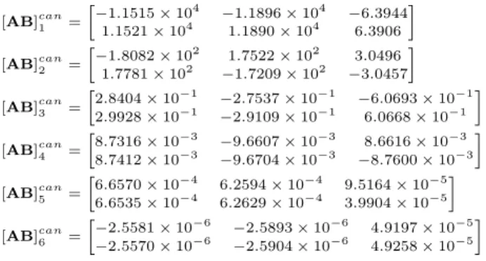
In the following, the components of the HOSVD based canonical form of the impedance model are introduced. The system is represented by the vertex models and the weighting functions. Let us partition the LTI vertices (Scanr ) as follows:
Scanr =
A B C D
. (12)
As the transformation results in C= [1 0]T and D= 0 for allτ ∈Ω, onlyA and Bare written in the list below:
[AB]can1 =
−1.1515×10⁴ −1.1896×10⁴ −6.3944 1.1521×10⁴ 1.1890×10⁴ 6.3906
[AB]can2 =
−1.8082×10² 1.7522×10² 3.0496 1.7781×10² −1.7209×10² −3.0457
[AB]can3 =
2.8404×10⁻¹ −2.7537×10⁻¹ −6.0693×10⁻¹ 2.9928×10⁻¹ −2.9109×10⁻¹ 6.0668×10⁻¹
[AB]can4 =
8.7316×10⁻³ −9.6607×10⁻³ 8.6616×10⁻³ 8.7412×10⁻³ −9.6704×10⁻³ −8.7600×10⁻³
[AB]can5 =
6.6570×10⁻⁴ 6.2594×10⁻⁴ 9.5164×10⁻⁵ 6.6535×10⁻⁴ 6.2629×10⁻⁴ 3.9904×10⁻⁵
[AB]can6 =
−2.5581×10⁻⁶ −2.5893×10⁻⁶ 4.9197×10⁻⁵
−2.5570×10⁻⁶ −2.5904×10⁻⁶ 4.9258×10⁻⁵
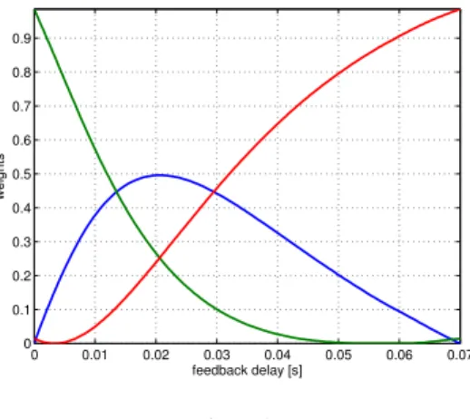
Figure 3 shows the weighting functionsw(τ)over the range of Ω. The smoothness of the weighting functions shows that the applied reidentification method is stable along the investigated range of τ. This means that the applied identification algo- rithm does not alternate between different local solutions (local minimums). It is worth mentioning that if the identification method is switching between different so- lutions, additional ranks could appear in the HOSVD canonical form. By neglecting the extra singular values, HOSVD is able to (smoothly) approximate the ruggedness in least-square sense in a way similar to how SVD can be used for noise filtering in digital signal processing [30]. However, if the fluctuation is large, such approxima- tion should be applied with circumspection.
0 0.01 0.02 0.03 0.04 0.05 0.06 0.07
−0.3
−0.2
−0.1 0 0.1 0.2
feedback delay [s]
weights
Figure 3
Weighting functions of the HOSVD based canonical form
4.2 Executing trade-off by TP model transformation
As was mentioned before, a trade-off can be determined between the complexity and the accuracy of the TP type polytopic model. The goal of this subsection is
to reveal the correlation between the accuracy and the number of utilized vertices.
Considering that the LMI based design process is very sensitive to the complexity of the polytopic model, it is very important to find the minimum complexity that reaches the accuracy threshold of the given engineering problem.
Even for the computational solutions of LMI toolbox for MATLAB that introduces high quality LMI solvers [31], the computational requirements explodes exponen- tially by the number of vertex models. Over a certain number of vertices, the LMI solvers may not be able to provide the solution. Considering that the significance of the vertex models decreases uniformly (Figure 2), there is no theoretically appeal- ing point from where to cut the less significant vertices to reduce the complexity of the model. However, a systematically executed trade-off could help to find the reasonable complexity. The HOSVD based canonical form readily supports a kind of principal component analysis of the investigated dynamical system model. In this analysis, the model accuracy is measured by the modeling errorǫr defined as:
ǫr=
SD(Ω,M)− SApproxD(Ω,M)
r
L
2
, (13)
where SD(Ω,M) can be computed using CHOSVD in the second step of the TP model transformation. SApproxD(Ω,M)
r is computed analogously but considers only the vertex models according to the first r singular values. Modeling errors result as follows:
ǫ1= 3.53×10²≤3.541×10² ǫ2= 1.0333≤1.0566
ǫ3= 2.22×10⁻²≤2.35×10⁻² ǫ4= 1.3×10⁻³≤1.4×10⁻³ ǫ5= 6.9808×10⁻⁵≤6.9808×10⁻⁵ ǫ6= 1.1272×10⁻¹¹≈0(numerically zero)
As matrix [AB]r contains element in the order of magnitude103, due to the defini- tion ofǫr,ǫ6is much larger then10−15, which is typically considered as numerically zero if all the matrix elements are in the range of101.ǫr is upper bounded by the sum of the singular values of the neglected vertices. The upper bounds are also displayed in the above list.
Figure 4(a) displays the modeling errors. One can see that the modeling error de- creases betweenǫ6andǫ5 much larger then in the case of the other reduction steps.
This measure describes the model accuracy only over the discrete delay values de- fined byM and does not give information about the correctness between the discrete points that have been used in the first step of the TP model transformation. To fol- low a more extensive investigation and to ensure that the resulted TP model is not under-sampled, let us define the following measure:
1 2 3 4 5 6 10−15
10−10 10−5 100 105
Keeping N singular value Modeling error εN
(a) Modelling error (ǫr) in function of dimension- ality of HOSVD based canonical form
1 2 3 4 5 6
10−2 10−1 100 101 102 103
Keeping N singular value Modeling error εRND1000 N
(b) Modelling error (ǫRN D1000r ) in function of di- mensionality of hosvd-based canonical form
Figure 4
Accuracy-complexity trade-off
Definition 11 (ǫRND1000r )
ǫRND1000r =
SD(Ω,M′)− SApproxD(Ω,M′)
r
L
2
, (14)
whereM′denotes a discretization grid with1000randomly generated grid points over Ω. GridM′is not equidistant andM′T
M =∅.
The measure ǫRND1000r compares the reidentified and the approximated systems in 1000randomly generated points considering the firstrvertices of the HOSVD based model. ǫRND1000r shows the model accuracy better in real situations where arbitrary varying delays occur. The resultedǫRND1000r s are listed below:
ǫRND10001 = 9.6325×10² ǫRND10002 = 2.7698 ǫRND10003 = 1.2099×10⁻¹ ǫRND10004 = 1.0519×10⁻¹ ǫRND10005 = 1.0514×10⁻¹ ǫRND10006 = 1.0514×10⁻¹
The values forr= 4,r= 5,r= 6are almost the same and start to increase only at
r= 3. Figure 4(b) displays the ǫRND1000r data in logarithmic scale and the big step byr= 3 is evident.
These results support the hypothesis that the number of non-zero singular values do not increase, even when the density ofM is increased without bounds. Thus, results show that the representation is minimal and exact. It can also be concluded that the applied discretization is not under-sampled, hence complexity reduction by ne- glecting the less significant vertices is well established. Beyond this pure numerical comparison, the dynamic accuracy of the TP model is also investigated in section 6.
5 Different convex TP model representations
As was already emphasized, LMIs are very sensitive to the shape of the convex hull that defines the polytopic qLPV representation together with the weighting functions.
Different types of convex hulls of the delayed impedance model can be generated utilizing the hull manipulation capabilities of TP model transformation. For the sake of brevity, only the non-exact, CNO type convex model with 3 vertices is detailed here. Even using the most developed optimization strategies, it is not possible to generate NO type convex hulls. From the engineering aspect, this hypothesis can be accepted since the CNO type convex hulls fulfill the requirements of control synthesis.
0 0.01 0.02 0.03 0.04 0.05 0.06 0.07
0 0.1 0.2 0.3 0.4 0.5 0.6 0.7 0.8 0.9
feedback delay [s]
weights
Figure 5
Weighting functions of CNO type convex hull of the reduced TP model with 3 vertices
[AB]cno31 =
9.7873×10² 1.0209×10³ 8.6644×10⁻¹
−9.7957×10² −1.0200×10³ −8.6591×10⁻¹
[AB]cno32 =
9.4943×10² 1.0519×10³ 1.0101
−9.5043×10² −1.0509×10³ −1.0091
[AB]cno33 =
1.0005×10³ 9.9947×10² 1.8247×10⁻¹
−1.0007×10³ −9.9929×10² −1.8254×10⁻¹
6 Analysis of the convex representation
The goal of this section is to illustrate the dynamical accuracy of the different TP models. Here the model accuracy is investigated by means of the difference between the step response of the polytopic model and the original delayed model. Due to the limited extent of this paper, only a set of practically interesting validation cases have been included. The comparison is broken into two parts according to the constant delay and varying delay cases.
6.1 Constant time-delay
Firstly, the dynamic accuracy of the HOSVD based canonical forms of the delayed impedance model with different complexity is examined. Figure 6 shows the step responses of the compared models at an arbitrarily chosen constant delay value (τ= 0.05567). As input signal, a 1N force step was used at 0.1s in the simulation.
Subfigures 6/a-f shows the step responses of TP models with a different number of neglected less significant vertices. The time plots confirm the result of the modeling error analysis done in 4.2. As the values ofǫRND1000r suggested, the TP models show similarly good accuracy with 6, 5 and 4 vertices and the model accuracy begins to relapse with 3 vertices. A TP model with 2 and only 1 vertices cannot describe the dynamics of the original delayed system properly.
For the purpose of confidence, the same simulations have been executed on CNO type TP models with 5, 4 and 3 vertices (Figure 7). As was expected, the time plots show the same result as the HOSVD based canonical type with equivalent complexities.
We can conclude that the CNO type TP models with 5,4 and 3 vertices give very similar responses independently from the complexity. The convex hull of the inves- tigated polytopic model cannot be formed with less then three vertices because the resulted domain of LPV models are not on the hyperline that can be defined by the convex combinations of two vertex systems. The results suggest that the CNO type convex TP model with 3 vertices provides sufficient accuracy for controller design purposes.
For the quantitative comparison, theL2 norm of the position error (the square root of sum of squares) and the maximum error is computed at four arbitrarily chosenτ values (neither of them are on the gridM) considering the1slong execution of the previously discussed simulation scenario. Results are displayed in Table 1.
0 0.2 0.4 0.6 0.8 1 0
0.1 0.2 0.3 0.4 0.5 0.6 0.7 0.8 0.9
1x 10⁻³
time [s]
position [m]
Original delayed model TP model
(a) Canonical form with 6 vertices (exact model)
0 0.2 0.4 0.6 0.8 1
0 0.1 0.2 0.3 0.4 0.5 0.6 0.7 0.8 0.9
1x 10⁻³
time [s]
position [m]
Original delayed model TP model
(b) Canonical form with 5 vertices
0 0.2 0.4 0.6 0.8 1
0 0.1 0.2 0.3 0.4 0.5 0.6 0.7 0.8 0.9
1x 10⁻³
time [s]
position [m]
Original delayed model TP model
(c) Canonical form with 4 vertices
0 0.2 0.4 0.6 0.8 1
0 0.1 0.2 0.3 0.4 0.5 0.6 0.7 0.8 0.9
1x 10⁻³
time [s]
position [m]
Original delayed model TP model
(d) Canonical form with 3 vertices
0 0.2 0.4 0.6 0.8 1
0 0.1 0.2 0.3 0.4 0.5 0.6 0.7 0.8 0.9
1x 10⁻³
time [s]
position [m]
Original delayed model TP model
(e) Canonical form with 2 vertices
0 0.2 0.4 0.6 0.8 1
0 0.1 0.2 0.3 0.4 0.5 0.6 0.7 0.8 0.9
1x 10⁻³
time [s]
position [m]
Original delayed model TP model
(f) Canonical form with 1 vertices
Figure 6
Comparison of the original delayed model and the HOSVD-based canonical form of the TP model with different complexity
0 0.2 0.4 0.6 0.8 1 0
0.1 0.2 0.3 0.4 0.5 0.6 0.7 0.8 0.9
1x 10⁻³
time [s]
position [m]
(a) CNO5
0 0.2 0.4 0.6 0.8 1
0 0.1 0.2 0.3 0.4 0.5 0.6 0.7 0.8 0.9
1x 10⁻³
time [s]
position [m]
(b) CNO4
0 0.2 0.4 0.6 0.8 1
0 0.1 0.2 0.3 0.4 0.5 0.6 0.7 0.8 0.9
1x 10⁻³
time [s]
position [m]
(c) CNO3
Figure 7
Comparison of the original delayed model and the CNO type TP model with different complexity
Table 1
Quantitative comparison of the original delayed model and the CNO type TP model with 3 vertices
L2 error M axerror τ = 0.01375s 2.6279×10⁻⁵ 9.8521×10⁻⁷ τ = 0.02941s 4.0380×10⁻⁵ 5.9765×10⁻⁶ τ = 0.04752s 4.3281×10⁻⁵ 1.0500×10⁻⁵ τ = 0.06393s 1.0851×10⁻⁴ 1.3048×10⁻⁵
6.2 Varying time-delay
The models have been compared under varying delay as well. The value ofτ(t)was varied as a sine function of timeτ(t) = 0.03 + sin(tπ)0.025. The input signal was a square wave with the frequency of2Hz and amplitude of1N. Figure 8 shows the result of the simulation.
Figure 8
Comparison under varying delay
Conclusion
In this paper the HOSVD based canonical form of the model of the generic impedance controlled actuation with feedback delay was determined via a TP model transforma- tion. A complexity trade off was also performed to determine non-exact TP models neglecting vertex systems with the less contribution. Via this investigation it has been proved that the TP model transformation is capable of manipulating the convex hull of the model wherein time delayτ appears as an external parameter. It has been shown that a convex polytop structure requires 6 vertex models for exact representa- tion of the investigated model for anyτ∈Ω. We presented the correlation between the number of vertex models and the number of singular values of the HOSVD based canonical form and the L2 norm based error of the polytopic structure over the transformation spaceΩ. In order to satisfy the basic requirements of LMI based design and further convex hull manipulation based optimization of the control design SNNN, IRNO and CNO type convex TP models was generated for the reduced 3 vertex model based convex hull.
Acknowledgement
The research was supported by the Hungarian National Development Agency, (ERC- HU-09-1-2009-0004 MTASZTAK) (OMFB-01677/2009).
References
[1] P. Baranyi, “TP model transformation as a way to LMI based controller de- sign,” IEEE Transaction on Industrial Electronics, vol. 51, pp. 387–400, April 2004.
[2] P. Baranyi, “Tensor-product model-based control of two-dimensional aeroelastic system,” Journal of Guidance, Control, and Dynamics, vol. 29, pp. 391–400, May-June 2005.
[3] P. Baranyi, “Output feedback control of two-dimensional aeroelastic system,”
Journal of Guidance, Control, and Dynamics, vol. 29, pp. 762–767, May-June 2005.
[4] F. Kolonic, A. Poljugan, and I. Petrovic, “Tensor product model transformation- based controller design for gantry crane control system - an application ap- proach,” Acta Polytechnica Hungarica, vol. 3, no. 4, pp. 95–112, 2006.
[5] R. Precup, L. Dioanca, E. M. Petriu, M. Radac, S. Preitl, and C. Dragos,
“Tensor product-based real-time control of the liquid levels in a three tank system,” in 2010 IEEE/ASME International Conference on Advanced Intelligent Mechatronics, (Montreal, QC, Canada), pp. 768–773, July 2010.
[6] Z. Szabó, P. Gáspár, and J. Bokor, “A novel control-oriented multi-affine qLPV modeling framework,” inControl Automation (MED), 2010 18th Mediterranean Conference on, pp. 1019–1024, June 2010.
[7] S. Ilea, J. Matusko, and F. Kolonic, “Tensor product transformation based speed control of permanent magnet synchronous motor drives,” in 17th International Conference on Electrical Drives and Power Electronics, EDPE 2011 (5th Joint Slovak-Croatian Conference), 2011.
[8] C. Sun, Y. Huang, C. Qian, and L. Wang, “On modeling and control of a flexible air-breathing hypersonic vehicle based on LPV method,” Frontiers of Electrical and Electronic Engineering, vol. 7, no. 1, pp. 56–68, 2012.
[9] T. Luspay, T. Péni, and B. Kulcsar, “Constrained freeway traffic control via lin- ear parameter varying paradigms,”Control of Linear Parameter Varying Systems With Applications, p. 461, 2012.
[10] B. Takarics and P. Baranyi, “Friction compensation in TP model form - aeroe- lastic wing as an example system,” Acta Polytechnica Hungarica, (Submitted).
[11] S. Chumalee and J. Whidborne,LPV Autopilot Design of a Jindivik UAV. Amer- ican Institute of Aeronautics and Astronautics, 1801 Alexander Bell Dr., Suite 500 Reston VA 20191-4344 USA„ 2009.
[12] S. Chumalee, Robust gain-scheduledH∞control for unmanned aerial vehicles.
PhD thesis, Cranfield University, Cranfield, UK, 2010.
[13] W. Qin, Z. Zheng, G. Liu, J. Ma, and W. Li, “Robust variable gain control for hypersonic vehicles based on LPV,” Systems Engineering and Electronics, vol. 33, no. 6, pp. 1327–1331, 2011.
[14] S. Rangajeeva and J. Whidborne, “Linear parameter varying control of a quadrotor,” in Industrial and Information Systems (ICIIS), 2011 6th IEEE Inter- national Conference on, pp. 483–488, Aug. 2011.
[15] W. Gai, H. Wang, T. Guo, and D. Li, “Modeling and LPV flight control of the canard rotor/ wing unmanned aerial vehicle,” inArtificial Intelligence, Man- agement Science and Electronic Commerce (AIMSEC), 2011 2nd International Conference on, pp. 2187–2191, Aug. 2011.
[16] R. Precup, C. Dragos, S. Preitl, M. Radac, and E. M. Petriu, “Novel tensor product models for automatic transmission system control,”IEEE Systems Jour- nal, p. In print., 2012.
[17] P. Baranyi, “Convex hull generation methods for polytopic representations of LPV models,” in Applied Machine Intelligence and Informatics, 2009. SAMI 2009. 7th International Symposium on, pp. 69–74, IEEE, 2009.
[18] P. Gróf, P. Baranyi, and P. Korondi, “Convex hull manipulation based control performance optimisation,”WSEAS Transactions on Systems and Control, vol. 5, pp. 691–700, August 2010.
[19] L. D. Lathauwer, B. D. Moor, and J. Vandewalle, “A multilinear singular value decomposition,” SIAM Journal on Matrix Analysis and Applications, vol. 21, no. 4, pp. 1253–1278, 2000.
[20] P. Baranyi, L. Szeidl, P. Várlaki, and Y. Yam, “Definition of the HOSVD-based canonical form of polytopic dynamic models,” in 3rd International Conference on Mechatronics (ICM 2006), (Budapest, Hungary), pp. 660–665, July 3-5 2006.
[21] L. Szeidl and P. Várlaki, “HOSVD based canonical form for polytopic mod- els of dynamic systems,” Journal of Advanced Computational Intelligence and Intelligent Informatics, vol. 13, no. 1, pp. 52–60, 2009.
[22] N. Hogan, “Impedance control: An approach to manipulation: Part I—Theory,”
Journal of Dynamic Systems, Measurement, and Control, vol. 107, pp. 1–7, Mar.
1985.
[23] N. Hogan, “Impedance control: An approach to manipulation: Part II—
Implementation,” Journal of Dynamic Systems, Measurement, and Control, vol. 107, pp. 8–16, Mar. 1985.
[24] N. Hogan, “Impedance control: An approach to manipulation: Part III—
Applications,”Journal of Dynamic Systems, Measurement, and Control, vol. 107, pp. 17–24, Mar. 1985.
[25] T. Hulin, C. Preusche, and G. Hirzinger, “Stability boundary for haptic ren- dering: Influence of physical damping,” inIntelligent Robots and Systems, 2006 IEEE/RSJ International Conference on, pp. 1570–1575, 2006.
[26] T. Hulin, C. Preusche, and G. Hirzinger, “Stability boundary for haptic ren- dering: Influence of human operator,” in Intelligent Robots and Systems, 2008.
IROS 2008. IEEE/RSJ International Conference on, pp. 3483–3488, 2008.
[27] J. J. Gil, E. Sanchez, T. Hulin, C. Preusche, and G. Hirzinger, “Stability bound- ary for haptic rendering: Influence of damping and delay,”Journal of Computing and Information Science in Engineering, vol. 9, pp. 011005–8, Mar. 2009.
[28] S. H. Kang, M. Jin, and P. H. Chang, “A solution to the Accuracy/Robustness dilemma in impedance control,” Mechatronics, IEEE/ASME Transactions on, vol. 14, no. 3, pp. 282–294, 2009.
[29] P. Galambos, P. Baranyi, and P. Korondi, “Extended TP model transformation for polytopic representation of impedance model with feedback delay,”WSEAS Transactions on Systems and Control, vol. 5, no. 9, pp. 701–710, 2010.
[30] E. Biglieri and K. Yao, “Some properties of singular value decomposition and their applications to digital signal processing,”Signal Processing, vol. 18, no. 3, pp. 277 – 289, 1989.
[31] Y. Nesterov and A. Nemirovskii, Interior-Point Polynomial Algorithms in Pro- gramming. Philadelphia: SIAM, 1994.