Obuda University ´
PhD Thesis
Closed-Loop Controller Design Possibilities for Nonlinear Physiological Systems
by
Gy¨ orgy Eigner Supervisor:
Prof. Dr. habil Levente Kov´ acs
Applied Informatics and Applied Mathematics Doctoral School
Budapest, 2017
Final Examination Committee:
Chair:
Prof. Dr. habil Aur´el Gal´antai, DSc Members:
Dr. M´arta Tak´acs, PhD Prof. Dr. habil P´eter Baranyi, DSc
Public Defense Committee:
Opponents:
Prof. Dr. Clara M. Ionescu, PhD (Ghent University, Belgium) Dr. Chee-Kong Chui, PhD (National University of Singapore, Singapore)
Chair:
Prof. Dr. S´andor Krist´aly, DSc Replacement Chair:
Prof. Dr. habil Aur´el Gal´antai, DSc Secretary:
Dr. P´eter Galambos, PhD Replacement Secretary / Member:
Dr. habil Gyula Hermann, CSc Members:
Dr. habil Szilveszter Kov´acs, PhD (University of Miskolc) Dr. Szilveszter Pletl, PhD (University of Szeged)
Dr. M´arta Tak´acs, PhD Replacement Member:
Dr. habil L´aszl´o Horv´ath, CSc
Date of Public Defense:
Declaration of Authorship
I, Gy¨orgy Eigner, declare that this thesis titled, ’Closed-Loop Controller Design Possibilities for Nonlinear Physiological Systems’ and the work presented in it are my own. I confirm that:
• This work was done while in candidature for a research degree at this University.
• Where I have consulted the published work of others, this is always clearly at- tributed.
• Where I have quoted from the work of others, the source is always given. With the exception of such quotations, this thesis is entirely my own work.
• I have acknowledged all main sources of help.
PhD Candidate
Date
”If we knew what we were doing, it wouldn’t be called research.”
Albert Einstein
Contents
1. Introduction 1
1.1. Research focus . . . 1
1.2. Relevant control engineering methods from this theses point of view . . . 5
1.3. Outline of this theses . . . 7
2. Opportunities of using Robust Fixed Point Transformation-based controller design in control of Diabetes Mellitus 9 2.1. Ideas which brought the RFPT-based control into life . . . 9
2.2. RFPT-based controller design in case of physiological processes . . . 13
2.2.1. Considered modeling difficulties in general . . . 13
2.2.2. Investigation of the effect chain of the control action . . . 14
2.2.3. Designing the approximate model. . . 15
2.2.4. Selection of the control law . . . 16
2.2.5. Finalization of the control environment . . . 16
2.2.6. Considerations and restrictions regarding the controller design in case of T1DM. . . 17
2.3. Control of T1DM via RFPT-based control framework . . . 18
2.3.1. Control of the Minimal model . . . 18
2.3.2. Control of the Cambridge (Hovorka) model . . . 25
2.3.3. Control of the UVA-Padova (Magni) model . . . 30
3. Novel perspective in the Control of Nonlinear Systems via a Linear Param- eter Varying method 39 3.1. Specificities of physiological LPV models . . . 39
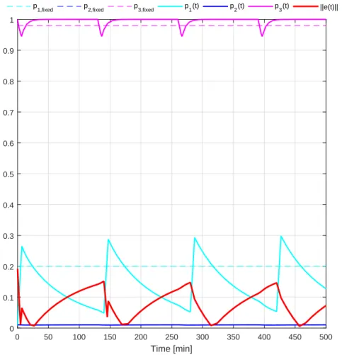
3.2. Different interpretations of quality based on LPV configurations . . . 41
3.2.1. Norm-based ”difference” definition in the parameter space . . . 42
3.2.2. Possible interpretations of the defined norm-based difference in the Parameter Space . . . 42
3.2.3. Usability of the development approach . . . 49
3.3. Novel completed controller scheme for LPV systems . . . 56
3.3.1. State feedback and gain-scheduling control . . . 56
3.3.2. Important properties of the investigated LPV system class. . . 57
3.3.3. Differences between the investigated LPV systems . . . 58
3.3.4. Mathematical background . . . 59
3.3.5. The completed feedback gain matrix . . . 60
3.3.6. Controller design, consequences and limitations . . . 62
3.4. Control of nonlinear physiological systems via competed LPV controller . 68 3.4.1. Control of nonlinear compartment model . . . 69
3.4.2. Control of T1DM . . . 73
3.4.3. Summary . . . 84
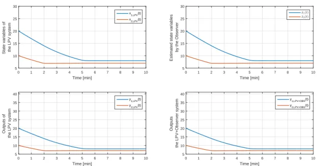
3.5. Observer based control for LPV systems . . . 85
3.5.1. Classical linear observer design . . . 85
3.5.2. Completed parameter dependent observer design . . . 86
3.5.3. Consequences, observer design and limitations . . . 86
3.6. Illustrative example for the completed observer structure. . . 88
3.6.1. Control of nonlinear compartmental model beside observer . . . . 88
3.6.2. Summary . . . 90
4. Tensor-Product model transformation based modeling 94 4.1. Motivation behind the usage of TP model transformation . . . 94
4.2. Theoretical background . . . 96
4.2.1. TP related mathematical tools . . . 96
4.3. Investigation of the TP-based modeling possibility of a nonlinear ICU diabetes model . . . 99
4.3.1. Derivation of the LPV and TP models . . . 99
4.3.2. TP models . . . 103
4.3.3. Validation of the generated models . . . 104
4.3.4. Summary . . . 109
4.4. Robustization possibilities via TP model framework . . . 110
4.4.1. Possible deviation-based qLPV and TP models . . . 110
4.4.2. Robustness of the models . . . 113
4.4.3. Validation . . . 115
4.4.4. Summary . . . 119
4.5. TP-modeling possibility for a complex T1DM model . . . 119
4.5.1. Steady state calculations. . . 120
4.5.2. qLPV Model derivation . . . 121
4.5.3. TP model form . . . 124
4.5.4. Validation . . . 124
4.5.5. Summary . . . 125
5. Conclusion 127
A. Summary of the new scientific results A-1
B. Detailed description of the used DM models B-1
B.1. Minimal Model . . . B-1 B.2. Model for Intensive Care Unit . . . B-3 B.2.1. The Wong model . . . B-3 B.3. Complex DM models . . . B-3 B.3.1. The Hovorka model . . . B-3 B.3.2. The Magni model . . . B-7
C. Physiological background and treatment C-1
C.1. Utilization of glucose . . . C-1 C.2. The Insulin . . . C-6 C.3. Types of the disease . . . C-10
C.3.1. Type 1 DM . . . C-10 C.3.2. Type 2 DM . . . C-11 C.3.3. Gestational DM . . . C-12 C.3.4. Double DM . . . C-12 C.3.5. Rare types . . . C-12 C.4. General side-effects of DM . . . C-12 C.5. Treatment possibilities . . . C-13 C.5.1. Prevention . . . C-14 C.5.2. Medication by drugs . . . C-14 C.5.3. Life-style therapies and diet . . . C-14 C.5.4. Intensive Conservative Therapy (ICT) . . . C-15 C.5.5. Insulin intake by insulin pen . . . C-15 C.5.6. Insulin intake by insulin pump . . . C-16
D. Linear Parameter Varying Systems C-1
D.1. Dynamical and LPV systems . . . C-1 D.1.1. State space representation of dynamic systems . . . C-1
D.1.2. State space representation of LPV systems . . . C-3
Acknowledgments
First of all, I would like to thank my doctoral supervisor, Prof. Levente Kov´acs – without his guidance and support from the beginning of my master studies this dissertation would not have been written. He believed in me when I was not and sometimes only his faith has been keeping my spirit up.
Next, I would like to special thank Prof. J´ozsef K. Tar, from whom I have learnt a lot not just professionally but also humanly – his help was eternally in order to finish this work.
After, I would also like to say thankProf. Imre Rudas– who has gave me extraordinary possibilities and embraced me.
I would like highlight my colleague Dr. Tam´as Ferenci, who provided me practical advices while I was writing the dissertation.
Special thanks behoove the leaders of the Doctoral School Prof. Aur´el Gal´antai and Prof. L´aszl´o Horv´ath for their support.
I want to say thanks to my family without they help this work would have been impossible – to my Mother-in-Law Kati and brother-in-law Benji; to Dr. Bernadett Eigner and Aunt Mary for their humanly and financial support; to mySisfor her kindness;
to my Grandma who always supported me; to my Dad for his encouragement; to my Mom for her continuous love and support.
I would like to also thank to all of those who are not personally listed here – many of my colleagues and friends from whom I learned a lot.
Finally, I would like to say special thanks to my beloved fianc´ee Barbi for her endless patience and love – as she always says this work would have been shorter but more boring without her.
List of Figures
1.1. Estimated number of people with diabetes worldwide and per region in 2015 and 2040 (20-79 years) [3] . . . 2 1.2. The AP concept [23] . . . 4 1.3. AP taxonomy - ”Solid lines demonstrate connections that are always
present and dashed lines represent connections that may only be present in some configurations. The tuning, model, and desired glucose concentration are all part of the controller, as signified by the black arrows. Green color distinguishes physiological states or properties from measured or digital signals. Black lines are used to indicate predetermined features of a block, and blue lines indicate signals or actions conducted during closed-loop operation” [20] ; Controller: MPC - Model Predictive Control, SC - Soft- Computing, PID - Proportional-Integral-Derivative Control, RB - Robust Control, FL - Fuzzy-rule based Control. . . 6 1.4. Structure of the thesis . . . 8 2.1. General RFPT controller scheme: the controller learns from the recent
model inputs and observed responses [qN(t) – Nominal trajectory; rd(t) – Desired system response; rdef(t) – Deformed system response; rr(t) – Realized system response; τ – Time shift] . . . 13 2.2. The scheme of the RFPT-based controller: the two delay blocks correspond
to the cycle time of the digital controller. . . 17 2.3. Results of the 48 hours long simulation with the Minimal model [GN = 85
mg/dL (4.675 mmol/L), Λ = 0.08,Ac= 1/10|Kc|,Kc=−200 and Bc= 1] 23 2.4. Results of the one week long simulations . . . 24 2.5. Results of the 48 hours long simulation of the Hovorka model [QN1 = 90
mmol/L (GN =QN1 /VG ≈ 8.036 mmol/L), Λ = 1e−4, Ac = 1/10|Kc|, Kc= 5e−1 andBc=−1] . . . 28 2.6. Results of the one week long simulations . . . 29 2.7. Effect chain of insulin . . . 31
2.8. Results of curve fittings based on (2.39) (for example, beside n = 0, R˜a = 0, ˜umin = 250 and ˜umax = 600), then ˜GM,stac(umin) ≈ 200 and G˜M,stac(umax) ≈ 40, the numerical calculation gives aest = −0.46 and best = 314.29).. . . 32 2.9. Result of a one week simulation with first feeding protocol [Control param-
eters: Λ = 0.015, Ac= 110−4,Kc=−1000, Bc= 1, Set-point (GN)=100 mg/dL ] . . . 35 2.10. Result of a 255 hours simulation with second feeding protocol [Control
parameters: Λ = 0.0125, Ac= 110−3,Kc =−1000, Bc =−1, Set-point (GN)=95 mg/dL ] . . . 36 2.11. Result of a 255 hours simulation with second feeding protocol [Control
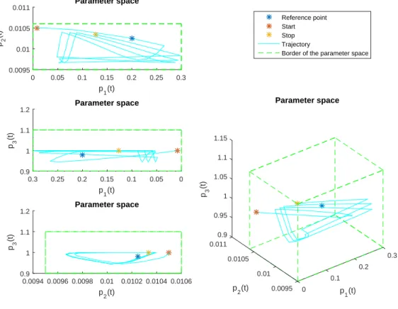
parameters: Λ = 0.0125, Ac= 110−3,Kc =−1000, Bc =−1, Set-point (GN)=95 mg/dL ] . . . 37 3.1. Examples of the possible interpretations of the 2-norm based difference. . 48 3.2. The outputs of the models . . . 51 3.3. Varying of the scheduling variables and the norm-based error signal . . . 52 3.4. Comparison of the magnitudes of the scheduling variables and the norm-
based error signal . . . 53 3.5. Evolution of the scheduling variables in the parameter space during operation 54 3.6. Different norm-based differences . . . 55 3.7. General feedback control loop with completed gain . . . 63 3.8. General feedback control loop with completed gain with feed forward
compensator . . . 64 3.9. General feedback control loop with completed gain in control oriented form 65 3.10. Nonlinear compartmental model . . . 70 3.11. Results of the simulation without control input saturations . . . 72 3.12. Results of the simulation with control input saturations . . . 73 3.13. General difference based completed controller structure with external
disturbance . . . 74 3.14. Finalized control environment with the original system, differnce based
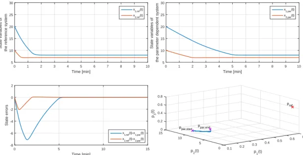
completed LPV controller with input virtualization and the mixed non- additive/additive EKF . . . 79 3.15. Comparison of the original system’s states and the estimated states (pro-
vided by the EKF) . . . 82 3.16. Results of the simulation of T1DM control, OoM: Order of Magnitude . . 83
3.17. General feedback control loop with completed observer and gain . . . 87 3.18. States and outputs of the controlled LPV and controlled and observed
LPV system . . . 90 3.19. Result of the simulations . . . 91 3.20. Parameter space and parameter errors. Upper row: PS of LPV system;
middle row: PS of the observer; lower row: parameter error . . . 92 4.1. Parameter space of a LPV system with defined parameter box (cube) and
Ωbounding simplex . . . 95 4.2. Weighting functions of the TP polytopic model. Left column: wn(p(t))Gd=GE,
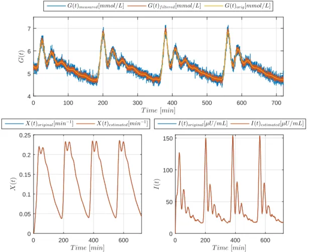
right column: wn(p(t))Gd6=GE. . . 104 4.3. 300 minutes long simulation in case of realistic inputs. . . 108 4.4. State error evolution over 300 minutes long simulation in case of realistic
inputs. . . 109 4.5. Weighting functions of the TP polytopic model; simple model case. Upper
diagram: T1DM case; Lower diagram: T2DM case. . . 112 4.6. Weighting functions of the TP polytopic model; robust model case. . . 115 4.7. Comparison of the original nonlinear models and the TP versions of them;
simple model case. Upper row: T1DM models; Lower row: T2DM models.117 4.8. Comparison of the original nonlinear models and the TP versions of them;
robust model case. Upper row: T1DM models; Lower row: T2DM models.
Parameters: p1 = 0.0266,p2= 0.0258, n= 0.2231. . . 119 4.9. Weighting functions regarding the Hovorka TP model . . . 124 4.10. Validation of the TP model . . . 125 C.1. Process of digestion and absorption of glucose, Credit: dream10f (left),
Austin Community College (right) [139,140] . . . C-2 C.2. Stoichiometry of aerobic respiration and most known fermentation types
in eucaryotic cell, Credit: Darekk2 [141] . . . C-3 C.3. The citric acid (Szentgy¨orgyi-Krebs) cycle, Credit: Narayenese [142] . . . C-4 C.4. Regulation of the utilization of glucose, Credit: Benjamin Cummings [143]C-5 C.5. Insulin production and secretion, Credit: Beta Cell Biology Consortium
[145] . . . C-7 C.6. Pulsating nature of insulin secretion [148] . . . C-8 C.7. Different types of insulin and their effect [151] . . . C-9
C.8. Effect of insulin on hepatic cells. Insulin binds to its receptor (1), which starts many protein activation cascades (2). These include translocation of Glut-4 transporter to the plasma membrane and influx of glucose (3), glycogen synthesis (4), glycolysis (5) and triglyceride synthesis (6)., Credit:
XcepticZP [152]. . . C-10 C.9. Insulin pen, Credit: UPMC [154] . . . C-16 C.10.Insulin pump, Credit: Mayo Clinic [155] . . . C-16 D.1. Affine LPV model example in the 3D parameter space . . . C-7 D.2. Polytopic LPV model examples in the 3Dparameter space . . . C-10
List of Tables
2.1. The randomized feed intake protocol . . . 22 4.1. Results of the RMSE-based investigations: RMSE-based comparison of
the states of the realized models on the given parameter domain under 100 minutes. Initial conditions: G0 = 15,Q0 = 3 and I0= 5. . . 106 4.2. Results of the RMSE-based investigations: RMSE-based comparison of
the states of the realized models on the given parameter domain under 300 minutes beside given impulse-kind inputs. Initial conditions: G0 = 15, Q0 = 3 andI0= 5 . . . 107 4.3. Results of the RMSE-based investigations. . . 114 4.4. Results of the RMSE-based investigations; simple model case. Initial
values: G0 = 100, X0 = 0, I0 = 11.5; simulation length: 150 min;
Sampling density in the parameter domain: 301. . . 116 4.5. Results of the RMSE-based investigations; robust model case. Initial
values: G0 = 100, X0 = 0, I0 = 11.5; simulation length: 300 min;
Sampling density in the parameter domain: G−301,p1−11,p2−11 and p3−11. . . 118 B.1. States, inputs and output of the used Minimal-model . . . B-2 B.2. Parameters and their details in the used Minimal-model . . . B-2 B.3. Detailed desriptions and values of the parameters of the Wong-model . . . B-4 B.4. States, inputs and output of the used Hovorka-model . . . B-6 B.5. Parameters and their details in the used Hovorka-model . . . B-7 B.6. States, inputs and output of the used Magni-model . . . B-10 B.7. Parameters and their details in the used Magni-model . . . B-11 B.8. Parameters and their details in the used Magni-model . . . B-12
Abstract
The usage of modeling and control on the field of biomedical engineering has essential importance in these days. The phenomena dates back to the occurrence of first high capacity computers with which the online monitoring, modeling and control became possible. Currently, several physiological processes can be handled by internal (eg.
pacemakers and other implants, etc.) and external (eg. heart-lung monitors, insulin pumps, etc.) controllers which provide accurate control signals with good quality – it can be stated that the modern medicine is unimaginable without these improvements.
One of the most widespread disease the diabetes mellitus and accompanying diseases, which mostly the side-effects of the main problem. Due to unknown autoimmune processes, civilizational reasons and most common genetic failures the diabetes mellitus threads significant part of the global population. The last decades have presented that via the biomedical engineering approaches and developments the diabetes mellitus can be sufficiently handled and the occurrence of side-effects can be decreased – thankfully the achievements on the field of physiological related modeling and control.
This dissertation presented modeling and control solutions which can be applied in case of physiological processes including diabetes mellitus.
The first thesis group investigated the usability of RFPT theorems in conjunction with T1DM control. I have examined three cases, which were different from the applied T1DM model, absorption submodel point of view, however, I used almost the same control strategies in each cases, namely, PID-kind control laws in the control block. I followed the general RFPT controller design steps, what I summarized at the beginning of the given chapter. The results showed that the RFPT-based controllers can be used in case of T1DM models with low and high complexity beside unfavorable disturbances (glucose loads). The developed controller were able to keep the BG level in the normal glycemic range; totally avoid hypoglycemia; however, short hyperglycemic periods occurred during the simulations. With this research I can be proven that the RFPT-based controller design method can be used for controller design in case of T1DM models with high nonlinearities.
The second thesis group introduce a two novel achievements on the field of LPV-based control. I have developed a norm based tool in which the norm (2-norm) is defined on the abstract parameter space of LPV systems and can be used as a metric between LTI systems. This tool can be used as error or difference metric and via quality requirements can be defined with it. The second achievement can be divided into two parts: I have
developed a novel LPV completed controller scheme which can be used for control of LPV (and trough nonlinear) systems with given properties; moreover, I have developed a completed LPV controller-observer scheme in order to control given LPV systems. The novel controller design tools are a mixture of linear state-feedback theorem and matrix similarity theorems and exploiting the properties of the LPV parameter space. I have proven the usability of the methods via nonlinear physiological examples including DM control. I provided deep analysis of the methods.
The third thesis group investigates the TP modeling possibilities of different DM models – due to I want to use the developed TP models as subjects for TP-based controller design in the future. The first step of this direction was made during my research, namely, I have introduced control oriented LPV models via mathematical transformation from the existing DM models and I successfully developed the TP model form of them. I showed three possible direction during this part: it is possible to use TP model transformation and realize TP model in case of simple ICU kind DM model with high nonlinearities;
it is possible to use TP model transformation and realize TP model in case of highly complex T1DM model with high nonlinearities and coupling; and I showed that how is it possible to increase the robustness of the TP model (from parameter point of view).
Absztrakt
A modellez´es ´es szab´alyoz´as haszn´alata az eg´eszs´eg¨ugyi m´ern¨oki ter¨uleten alapvet˝o fontoss´aggal b´ır napjainkban. A jelens´eg visszadat´alhat´o az els˝o nagy teljesitmeny˝u szamit´og´epek megjelen´es´ere, amelyekkel az online monitoroz´as, modellez´es ´es szab´alyoz´as tervez´es megval´os´ıthat´ov´a v´alt. Manaps´ag sz´amos ´elettani folyamat szab´alyozhat´o bels˝o (pl. pacemaker ´es egy´eb implant´atumok, stb.) vagy k¨uls˝o (pl. sz´ıv-t¨ud˝o monitor, inzulin pumpa, stb.) szab´alyoz´okkal, amelyek pontos ´es j´o min˝os´eg˝u szab´alyoz´ast tesznek lehet˝ove – kijenelthetj¨uk, hogy a modern medic´ına elk´epzelhetetlen lenne ezen fejleszt´esek nelk¨ul.
Az egyik legelterjedtebb k´or a cukorbetegs´eg ´es ennek mell´ekhat´asak´ent kialakul´o t´arsult betegs´egek. Az ismeretlen autoimmun folyamatok, civiliz´aci´os hat´asok ´es genetikai betegs´egek k¨ovetkezt´eben kialakul´o cukorbetegs´eg a glob´alis popul´aci´o jelent˝os r´esz´et fenyegeti. Az elm´ult ´evtizedekben bebizonyosodott, hogy az eg´eszs´eg¨ugyi m´ern¨oki megold´asokkal a cukorbetegs´eg hat´ekonyan kezelhet˝o ´es a t´arsult betegs´egek el˝ofordul´as´anak gyakoris´aga is reduk´alhat´o – k¨osz¨onhet˝oen a sz´amos ´uj eredm´enynek a fiziol´ogiai rendsz- erek modellez´es´evel ´es szab´alyoz´as´aval kapcsolatban.
Ez a disszert´aci´o olyan modellez´esi ´es szab´alyoz´asi megold´asokat mutat be, amelyek haszn´alhat´oak az ´elattani folyamatokkal kapcsolatosan, bele´ertve a cukorbetegs´eget is.
Az els˝o t´ezis csoportban megvizsg´altam a Robusztus Fix-Pont Transzform´aci´o (RFPT)- alap´u szab´alyoz´as tervez´esi lehet˝os´egeket egyes t´ıpus´u DM (T1DM) szab´alyoz´as´aval kapcsolatban. H´arom esetet vettem vizsg´alat al´a, amelyek az alkalmazott T1DM modell
´es felsz´ıv´od´asi modell tekintet´eben k¨ul¨onb¨oz˝ok voltak, azonban a haszn´alt szab´alyozasi strat´egia, vagyis a Proporcion´alis-Integr´al´o-Deriv´al´o (PID)-alap´u szab´alyoz´asi t¨orv´eny a szab´alyoz´o blokkban ugyanazon elven alapult. Az ´altal´anos RFPT tervez´esi l´ep´eseket k¨ovettem, amelyeket ¨osszefoglal´oan megadtam fiziol´ogiai rendszerek eset´ere a fejezet elej´en.
Az eredm´enyek memutatt´ak, hogy az RFPT-alap´u szab´alyoz´ok haszn´alh´at´oak alacsony
´es magasrend˝u T1DM modellek szab´alyoz´as´ahoz nagymertek˝u zavar´as (nagym´ertek˝u sz´enhidr´at (CHO) terhel´es) mellett. A kifejlesztett szab´alyoz´asok a szimul´aci´os id˝o alatt k´epesek voltak a v´ercukor szintet norm´al glik´emi´as tartom´anyban tartani; teljesen elker¨ulni a hypoglik´emi´as epiz´odokat; hab´ar r¨ovid idej˝u hyperglik´emi´as epiz´od´ok el˝ofordultak. Ezzel a kutat´assal siker¨ult bizony´ıtanom, hogy az RFPT-alap´u szab´alyoz´o tervez´esi elj´ar´asok haszn´alhat´oak szab´alyoz´ok tervez´es´ere nagymertek˝u nemlinearit´asokkal rendelkez˝o T1DM modellekhez.
A m´asodik t´eziscsoportban k´et ´uj, eredeti eredm´enyemet mutatom be a line´aris pa- rameterv´altoz´os rendszer (LPV)-alap´u szabalyoz´asok ter¨ulet´er˝ol. Kifejlesztettem egy
norma alap´u eszk¨ozt, ahol a norma (2-es norma) az LPV rendszerek absztrakt param´eter ter´en ´ertelmezve metrikak´ent hasznalhat´o LTI rendszerek k¨oz¨ott. Ez az eszk¨oz alkalmas hiba- vagy k¨ul¨onbs´eg-metrikak´ent val´o haszn´alatra is ´es ´altala min˝os´egi k¨ovetelm´enyek is megfogalmazhat´oak. A m´asodik fejleszt´es k´et r´eszre oszthat´o: kifejlesztettem egy ´uj LPV kiegesz´ıtett szab´alyoz´o s´em´at, amely LPV rendszerek szab´alyoz´as´ahoz haszn´alhat´o fel;
tov´abb´a, egy ´uj, kieg´esz´ıtett LPV szab´alyoz´o-megfigyel˝o strukt´ur´at is fejlesztettem LPV rendszerek szab´alyoz´as´ahoz. Az ´uj eszk¨oz¨ok egy kever´ek´et alkotj´ak a line´aris ´allapot- visszacsatol´as alap´u szab´alyoz´asnak ´es a m´atrix hasonl´os´agi t´eteleknek ´es kihaszn´alj´ak az LPV param´eter t´er tulajdons´agait. Bebizony´ıtottam a haszn´alhat´os´agukat nem- line´aris fiziol´ogiai p´eld´akon kereszt¨ul, bele´ertve a diabetes mellitusz (DM) szab´alyoz´ast is.
Elv´egeztem az eszk¨oz¨ok teljesk¨or˝u anal´ızis´et is.
A harmadik t´eziscsoportban a tenzor szorzat (TP)-alap´u modellez´esi lehet˝os´egeket vizsg´altam meg k¨ul¨onb¨oz˝o DM modellek eset´en – mivel ezeket a realiz´alt TP modelleket akarom felhaszn´alni a tov´abbi TP-alap´u szab´alyoz´astervez´esi kutat´asokhoz. Ennek az els˝o l´ep´ese ker¨ult kidolgoz´asra a kutat´asomban, azaz bevezettem letez˝o DM modellek kontroll- orient´alt LPV v´altozatait matematikai transzform´aci´okon kereszt¨ul, majd ezeken sikeresen alkalmaztam a TP model transzformaci´ot el˝o´all´ıtva TP-alap´u modelljeiket. H´arom lehets´eges ir´anyt v´azoltam fel: bemutattam, hogy lehets´eges a TP-model transzform´aci´o haszn´alata TP modellek realiz´al´as´ahoz egyszer˝u, intenz´ıv ˝orz˝okre szabott (ICU) DM modell eset´en, amely nagym´ert´ek˝u nemlinearit´asokkal rendelkezik; lehets´eges a TP-model transzform´aci´o haszn´alata TP modellek realiz´al´as´ahoz komplex T1DM modell eset´en, amely nagym´ert´ek˝u nemlinearit´asokkal es csatol´asokkal rendelkezik; ´es megmutattam, hogy lehets´eges a TP modell robusztiz´al´asa modell param´eterek szempontj´ab´ol.
List of abbreviations
Abbreviation Meaning
LTI Linear Time Invariant
LTV Linear Time Variant
NLTV Nonlinear LTV
LPV Linear Parameter Varying
qLPV quasi LPV
TP model Tensor Product model
SS State Space
PS Parameter Space
PB Parameter Box
DM Diabetes Mellitus
CHO Carbohydrate
LMI Linear Matrix Inequality LQR Linear Quadratic Regulation
MVS Minimal Volume Simplex
SVD Singular Value Decomposition
HOSVD Higher-Order SVD
AP Artificial Pancreas
T1DM Type 1 DM
T2DM Type 2 DM
List of mathematical notations
Notation Meaning
a, b, ... scalars a,b, ... vector A,B, ... matrices
ai,bi, ... ith row vector of A,B, ... matrices ai,j, bi,j, ... jth elements of the ai,i, ...row vectors R,C sets
A,B, ... tensors S N
n=1wn multiple tensor products, e.g. S ×1w1...×NwN
1. Introduction
1.1. Research focus
The aim of this theses is to introduce such kind of modeling and controller design solutions which can be used in case of nonlinear biological systems. Each proposed methods are universal ones and can be used in case of arbitrary nonlinear processes, however, the application of them is unique in the current research field.
My main motivating goal was the use of the developments and applications in the research of DM from engineering point of view - in this spirit I always kept in the focus how the reached results will be useful to reach this goal. Namely, how can the proposed techniques be applied in case of DM.
Modeling and control is extremely important in the artificial regulation of physiological processes, especially where the good quality of external control is a must [1]. However, the given field is loaded by several challenges. Most of them are highly nonlinear, poorly described in full aspects due to the multiple and diverse connections between the physiological systems, deep investigations and measurements cannot be done or possible but with hard constraints, etc. [2]. Although these facts, the evolution and process of different types of DM became well described in the recent decades [3].
DM is a serious, chronic disease connected to the metabolic system of the human body. The disease occurs either when the amount of insulin produced by the pancreas is insufficient or when the body cannot effectively use the insulin it produces [4].
Insulin is the key hormone of the blood glucose regulation produced by the β-cells in the Langerhans-islets in the pancreas [5]. It makes possible the entering of the glucose into the glucose consuming body cells. Most of the cells feast glucose which is the major energy source in living organisms [6].
DM researches are hot topics on the biomedical engineering field due to the dramatically increasing number of diabetic patients. According to the newest estimations of the International Diabetes Federation (IDF) for the number of people who live with such form of diagnosed and undiagnosed DM is about 415 million worldwide in 2015 [3].
Furthermore, the short term prospects suggest that this number can be reached the 642
million, around 6.8% of the expected global population by 2040 [3, 4]. Figure1.1. shows the estimated distribution of diabetic population worldwide.
Figure 1.1.: Estimated number of people with diabetes worldwide and per region in 2015 and 2040 (20-79 years) [3]
DM is classified into Type 1 DM (T1DM), Type 2 DM (T2DM), Gestational DM, Double DM, Genetic DM, Secondary DM, etc. [3,7]. Despite the several different types of DM, the T1DM and T2DM are the most widespread.
The T1DM is related to the insulin hormone, since during the emergence of the disorder, the insulin producerβ-cells are burned out due to intense autoimmune reaction in which the patient’s own immune cells destroy them. The occurrence of T1DM is around 10% in the diabetic population [7].
The most common type of DM is T2DM [3]. The incidence of it is around 90% in the diabetic population. The disease evolves over longer period in the patients body.
However, the body is able to produce insulin internally, the body cells become resistant to the hormone and the effect of it becomes insufficient. Over long period persistent hyperglycemia and increasing insulin resistance can be observed [5,8].
A frequently occurred DM type is the Gestational DM, which appears in women during pregnancy. Most of the time it disappear after childbirth, however, the state can become permanent in case of genetic flair for DM [4].
The other types are rarely occurred in the population [3].
Important that the DM state can leads to several secondary disease in the absence of appropriate therapy, which means not just proper medication, but the change of lifestyle, as well.
The required therapies to handle the diabetic state are different in accordance the given type of DM. In case of T1DM the patients need exogenous administered insulin due to the lack of internally produced insulin. In case of T2DM, the regular therapy starts with drug administration. These can be gluconeogenesis inhibitors which obstruct the daily glucose production of the liver and decrease the insulin resistance [6]. Although, over time externally administered insulin can be required in order to keep the blood glucose level in a healthy range.
The common therapy - beside prescription about the lifestyle (physical activities and diet) - is the external insulin administration. Insulin is delivered via subcutaneous injections. There are different devices with which the diabetic patients can manage the insulin delivery. Usually, it is done by insulin pen which is a small pen shape mechanical device which consists of dispenser, insulin reservoir, injection mechanics and thin needle parts. In this way with this device the patients are able to manage their blood glucose level. The dosage is manual and leaves the insulin delivery to the patients based on preliminary rules laid down, the feed intake, physical activities and the prescription of the clinicians. During the self-administered therapy, the patients can use rapid acting insulin (bolus insulin to handle the feed intake) and slowly acting insulin (for keep the basal insulin rate), as well [7,9].
An other solution for insulin administration is the semi-automatic or automatic insulin pump or Continuous Subcutaneous Insulin Infusion (CSII) devices, which can be used both DM cases as well, however, the indications of usage are different [10–14]. The pump or injection system contains insulin reservoir which connects to the subcutaneous regions via thin catheter. This electromechanical devices are able to delivery insulin boluses automatically based on predefined rules. The pumps using rapid acting insulin and the delivery protocols are varying as demands the patients need.
The long term goal of the research of DM from engineering point of view is to develop the so-called Artificial Pancreas (AP) concept (Fig. 1.2). This development consist of three major part [15–21]:
1. An insulin pump or insulin pump completed with external insulin injection system,
which stores and injects the rapid acting insulin;
2. A Continuous Glucose Monitoring System (CGMS) for continuous blood sugar level measurement and transmit;
3. Appropriate software components including control algorithms, user interfaces, drivers.
The CGMS system is used in parallel with the insulin pump. The operation of CGMS are based on various principles. In practice, the most widely used systems are external devices fixed on the abdominal skin surface and connected to the subcutaneous level through a thin catheter. The most frequent measuring principle are enzymatic based (Glucose Oxidase (GOx)). Beside its several benefits CGMS has also some disadvantages mostly from control engineering point of view: sensors measurements are done only every 5 minutes. Implantable CGMS have been also appeared, but these are not available on the market, yet [22].
Figure 1.2.: The AP concept [23]
The newest concepts calculate with the benefits of the available smart devices, like smartphones [18]. In this way the control algorithms which may need high computational
capacity can be exported to the smart device instead of the compact insulin pumps.
Figure 1.2. shows the schematic representation of the latest AP concept.
As mentioned above, the third necessary component to realize the AP is the appropriate software elements, including the control algorithms, the ”soul” of this approach.
Due to the fact that insulin pump therapies are used mostly in case of T1DM, the advanced control algorithms developed inside AP researches focus on this DM form. The main expectation from an AP control algorithm is the automatic glucose regulation in order to keep the blood glucose concentration in the normal glycemic range, i.e. 70-110 mg/dL (3.9-6 mmol/L) and relying if possible on the compliance of the patient. The ultimate goal is to avoid the dangerously low blood glucose levels (massive hypoglycemia) that could directly endanger the patients’ life.
1.2. Relevant control engineering methods from this theses point of view
In this section I introduce the most important control design techniques from the DM and more specifically from the AP concept point of view – correspondingly to the aforementioned aims of the theses.
The soul of the AP concept is the usage of appropriate control algorithms. Over the last decades, most of the available control concepts have tested on this field. Figure 1.3 shows the AP concept completed with the most frequently used control algorithms.
The most important directions focus on model predictive control (MPC), fuzzy rule- based and other soft computing techniques, classical, robust and fractional PID control techniques; however, without having yet a general solution on the problem [15–17, 20, 21, 24].
Simplistically, every control algorithm considers similar principles; namely, the ful- fillment of prescribed quality and quantity properties. The first attempts on this area were related to ”Proportional-Integral-Derivative (PID)” control being still the most widely used classical control technique in the industry. Although the basic concept of PID control is not too sophisticated, highly advanced solutions like robust PID [20, 25] or switching PID [26,27] have been applied for the AP concept. Fractional PID control is in the mainframe of the physiological related control tasks [28]. There is example regarding to the application of fractional PID in the research field, like [29], but the usage as a common technique is not usual in the research field, however.
Figure 1.3.: AP taxonomy - ”Solid lines demonstrate connections that are always present and dashed lines represent connections that may only be present in some configurations. The tuning, model, and desired glucose concentration are all part of the controller, as signified by the black arrows. Green color distinguishes physiological states or properties from measured or digital signals.
Black lines are used to indicate predetermined features of a block, and blue lines indicate signals or actions conducted during closed-loop operation” [20]
; Controller: MPC - Model Predictive Control, SC - Soft-Computing, PID - Proportional-Integral-Derivative Control, RB - Robust Control, FL - Fuzzy- rule based Control
The MPC based solutions are widely used successfully since almost thirty years ago in the control engineering [30–33] and in physiological related context as well [34–36].
MPC techniques represent probably the mostly used advanced control method in the AP concept, but they suffers from intra- and inter-patient variabilities and external noises. MPC is a model based solution meaning that the controller tuning is based on the properties of a mathematical model (called nominal model). Nonetheless, MPC algorithms produce the best results in individual therapy with considering closely ideal conditions. Several, highly developed MPC based control solutions appeared in the recent years like Robust MPC (RMPC), Nonlinear MPC (NMPC), Robust, Nonlinear MPC (RNMPC), MPC with moving horizon [37–40]. One of the most straightforward
direction is the MPC design by using soft computing tuning tools [41]. The latter technique was successfully implemented on embedded systems which is a part of an artificial implementable AP [42].
Soft computing methodologies have been applied also several times in the AP concept, but only in the recent years have been investigated in clinical trials [43–45].
Modern robust control methods likeL2- orH∞-based ones were introduced in the AP researches in order to stave off the determinative uncertainties coming from inter- and intra-patient variability. Supplemented by LPV methodology (providing the opportunity to handle the original nonlinear system/model as a linear one; hence, to give access using the original nonlinear model for linear control methods enumerated above), modern robust control successfully deals with the quality and quantity requirements [46–49]. Another useful direction in this domain proved to be the combination of LPV methodologies with LMI-based one [49–51].
Dual hormone controllers consider beside the insulin the glucagon hormone as well;
hence, it represents another conceptual control approach in AP researches [52]. Clinical trials also stared in this direction with encouraging results [53].
1.3. Outline of this theses
In Chapter 2., I introduce the latest results on the field of adaptive robust control of T1DM via RFPT framework. Beside the introduction, I demonstrate the developments applying on sophisticated T1DM models.
Chapter 3. presents the development of a new quality marker (”metric”) for LPV modeling and control based on a given norm interpreted on the LPV parameter space.
Further, a novel completed LPV controller and observer scheme for nonlinear systems is proposed, which can be used in control of biomedical systems. The applicability of them are demonstrated on nonlinear compartmental and different DM models. Most of the widely used DM models are based on compartmental modeling due to an applied nonlinear physiological compartmental model is used for demonstration.
Chapter 4 details the TP modeling possibilities regarding to DM in order to realize control oriented LPV-TP models, which will be the subjects of the controller design later.
In Chapter5., I conclude my presented results.
Four Appendix encloses the theses. Appendix A. is a summary of the thesis points;
Appendix B. summarizes the description and parameters of the DM model which were used; AppendixC. summarizes of the DM and the current state-of-the art of the research of it; and AppendixD. introduces the types of the LPV systems which were applied in
the thesis.
The simplified structure and the interconnections between the Chapters and Appendices are presented by Fig. 1.4.
Ch. 1. Introduction
Ch. 2. RFPT-based control
Ch. 3. LPV-based tools
Ch. 4. TP-based modeling
App. 1. Summary of the thesis points App. 2. Used DM models
App. 3. DM summary App. 4. LPV systems
Ch. 5. Conclusion RFPT theorem
Design procedure of physiology related RFPT controller Control examples
Physology related LPV models Norm-based metric for LPV systems
Completed LPV controller design and examples Completed LPV observer design and example Theorem of the TP model transformation TP modeling examples
Figure 1.4.: Structure of the thesis
2. Opportunities of using Robust Fixed Point Transformation-based controller design in control of Diabetes Mellitus
In this Chapter, I have detailed my results concerning the application possibilities of the RFPT-based control theorem for control of T1DM.
First, I present the main ideas behind the RFPT-based control theorem.
Second, I describe the general method which can be used to realize the RFPT-based controllers which are able to deal with control of physiological models.
After, I have presented three case studies regarding the control of T1DM for models that are diverse from complexity, nonlinearity, structure and other points of view.
Finally, it should be noted that I have used ExcelTM for some calculations and SCILABTM for the simulation part, however, the figures were made by MATLABTM.
2.1. Ideas which brought the RFPT-based control into life
In control engineering the use of high complexity models have significant practical disadvantages. Typical problem is the reliability of the model parameters for the particular person under control. Furthermore, such models are difficult to handle. The traditional design methodologies formulate the feedback by the use of the actual system state in the given moment. In practice it is often impossible to obtain satisfactory information on the system’s actual state variable as a whole, only its certain components can be measured, either directly or indirectly. In the latter case, complicated model-based state estimation processes should be applied for the computation of the control signal. However, we are often lacking the necessary sensors.
A possible choice to handle these circumstances is the usage of Lyapunov’s methods.
Before the famous work of Lyapunov in the end of the 19th century, the scientist who was investigating the stability of nonlinear systems had to face with many challenges.
Lyapunov’s work provided a universal mathematical tool which let the researchers to decide whether a nonlinear system is stable or not [54,55]. Lyapunov’s second or direct
method provides a way to determine the stability of a nonlinear system without solving the equations of motion. Due to the fact that most of the real life problems do not have analytical solutions in closed form and the validity of numerical solutions is limited, Lyapunov’s method is extremely useful and most of the controller design methods are based on that even today.
The heart of the method is the evolution of the properties of the so-called Lyapunov functionV(t, x) over time. Consider a general nonlinear dynamic system, whereξ = 0 is an equilibrium point:
x(t) =˙ f(t, x) f(t,0) = 0 f(t, x)∈Ct,x(0,1) . (2.1) If, ∃V(t, x)∈Ct,x(1,1)([a,∞)×Dx) positive definite Lyapunov function that alongside
∀x(t) trajectories
V˙(t, x) = dV(t, x)
dt <0 ( ˙V negative definite) (2.2) thenξ = 0 solution (equilibrium) is asymptotically stable in Lyapunov sense [56].
Nevertheless, the use of this method has several drawbacks. Although Lyapunov’s method makes it possible to guarantee the asymptotic stability of various nonlinear systems, it does not provide information on the subtle details of the stabilization process.
The transients in the motion of the controlled systems normally remain obscure and may contain practically intolerable sessions. Mathematically it is hard to handle, and it has strict limitations. There are only a few rules of thumb and examples, therefore its application or adaptation to a given problem requires the highly creative thinking of an expert designer. Each nonlinear problem needs unique approach. Moreover, often direct measurements or state estimations are needed for the feedback which is not possible in the given circumstances.
In classical control theorems, for example PID or state feedback based controls, the control rule and action is based on the expected-observed control scheme. That means, we have a predefined or ”desired” system behavior rd and the purpose of the control action via the control signaluis to enforce the systemϕto reach the desired behavior. If the observed behavior differs from the desired one, error signals emerge in the trajectory tracking. The classical Model Predictive Controllers try to compensate them by error feedback terms on the basis of the assumption that they are in the possession of ”exact system models”. In other words, instead of directly concentrating on the response error, they rather observe only their consequences, and try to eliminate them on the basis of a not completely correct hypotheses. However, real physiological and physical systems can
be modeled only approximately [57]. In classical control theorems, the control goal can be formulated as:
rr =ϕ(u) , (2.3)
whererr is the actual (realized) system response afteru affected on it. In this case, the control signal calculation via exact inverse model can be described as:
ud=ϕ−1(rr) , (2.4)
where ud is the desired control signal to be applied in order to reach the rr system response.
In contrast to the Lyapunov method or classical control, the RFPT-based controller design has many advantages. It focuses on the kinematics of the motion which may have more importance than the global asymptotic stability; it does not require precise model of the controlled process, just an approximate one may do well (may be as highly approximate that the state feedback may become unimportant); the parameter uncertainties are well tolerated; and finally, the realization of the method is easier alongside certain given steps.
The main importance is that the RFPT theorem calculates with the high approximation of the given process and turns this property to a benefit. In the absence of exact models, approximate model can be used to describe the approximate control signal:
udappr =ϕ−1appr(rd) , (2.5) whereudappr is the approximate control signal which is necessary to reach therddesired system response.
Hence, the connection between the realized response rr and the desired responserd of the system can be described as:
rr ≡ϕ(ϕ−1appr(rd))≡f(rd)6=rd . (2.6) The RFPT-based adaptive control is just a possible alternative to the traditional approaches. This approach sharply distinguishes between the ”kinematic” and the
”dynamic” aspects.
It starts with a purely kinematically formulated trajectory tracking error relaxation strategy. This results a given order time-derivative of certain variables as desired system response rd that instantaneously can be realized by the available control signal. This control signal is estimated by the use of the available approximate system modelϕ−1appr
and it is exerted on the controlled systemϕ. The realized responserr of the controlled system that is obtained for a kinematic prescriptionr can be considered as a response function as f(r, . . .) in which the symbol ”. . .” refers to the parameters of the exact and the approximate system models. Evidentlyr and f(r) have the same dimensions and they need not comprise all the components of the state variable. In practical cases the complexity of the approximate model may be much lower than the exact model.
The basic idea is that instead of tuning the parameters of the approximate model, the kinematically prescribed rd value is adaptively deformed to r? so that rd =f(r?).
The necessary deformation is constructed in the following manner: in the first step the control problem is transformed into a fixed point problem so that the solution of the control task is its fixed point. After that, an iterative sequence of control signals is generated by the digital controller as{r0def= rd, r1 =G(r0). . . , rn+1=G(rn), . . .}. If the parameters of the transformation functionG are well set then this sequence converges to the solution of the control task, i.e. rn → r?. Normally rd depends only on the lower order time-derivatives of the considered state variables while r can be abruptly modified.
Therefore, although during one digital cycle only one step of iteration can be done, in the practice acceptable convergence can be achieved.
The idea of transforming various problems into fixed point problems is not a novel one. It goes back to the 17th century e.g. in the Newton-Raphson method [58–60]. Such kind of methods often occur in adaptive control as well [61,62]. In 1922 Stefan Banach generalized the method for linear, normed, complete metric spaces [63] via the application of contractive maps. In this case, in which the response function is a single-variable real function, the transformation is made by the function [64]:
rn+1=G(rn;rd)def= (rn+Kc)×
1 +Bchtanh(Ac(f(rn)−rd))i
−Kc , (2.7) where Kc, Ac, andBc(Bc=±1) are theadaptive control parameters. Clearly we have two fixed points as r =−Kc (that is trivial and useless for the controller), and r? for whichf(r?) =rd, that is the solution of the control task. If
dG dr
<1 during the iteration then the appropriate sequence converges to the solution of the control task. In general it is not difficult to satisfy this condition within a bounded region of the response values by manipulating the two parametersKc andAc. (Further details regarding the appropriate setting of the control parameters was given in [64,65]).
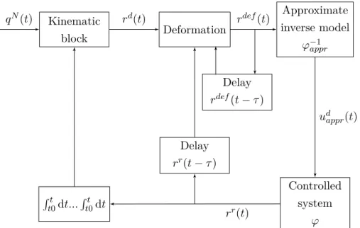
The general RFPT controller structure can be seen on Fig. 2.1.
Kinematic
block Deformation
Delay rdef(t−τ)
Delay rr(t−τ) Rt
t0dt...Rt0t dt
Approximate inverse model
ϕ−1appr
Controlled system
ϕ
qN(t) rd(t) rdef(t)
udappr(t)
rr(t)
Figure 2.1.: General RFPT controller scheme: the controller learns from the recent model inputs and observed responses [qN(t) – Nominal trajectory;rd(t) – Desired system response;rdef(t) – Deformed system response;rr(t) – Realized system response; τ – Time shift]
2.2. RFPT-based controller design in case of physiological processes
In this Section, I analyze the main steps of the controller design procedure starting with the general properties of the mathematical model of the phenomenon that I wish to use in the control. By revealing the more specific model properties an effect chain can be deduced that determines the relative order of the control tasks. By the use of a simple approximate model, the need for the information on the components of certain state variables can be evaded. The adaptivity of the designed controller can compensate the consequences of this modeling imprecision.
2.2.1. Considered modeling difficulties in general
In diabetes research, mathematical modeling of the physiological processes and the in- vitro investigations have absolute relevance due to the fact that the in-vivo experimenting possibility is limited since the subjects of the examinations are human beings. In such investigations, the real patients are substituted with models of various complexity called
”patient models”. These can be completed with other sub-models (e.g.: absorption
model, sensor model, noise model, etc.) in order to simulate the behavior of the human metabolic system regarding the glucose-insulin household. However, when the available mathematical models are used during the controller design, several unfavorable model properties come to light such as strong non-linearities and time delay effects that are essential parts of the reality [1]. Efficient handling of the intra- and inter- patient variabilities is also challenging, since a virtual patient can be described with a given parameter set of the mathematical model. Identification of the models is also crucial. Because of the inputs have impulse nature (food boluses, insulin injections), the aforementioned variabilities cannot be determined a priori. The output values are provided by real physiological measurements, therefore they are available only in given time moments. Furthermore, an identified individualized virtual patient model belongs only to a given real patient. That means that the model-based controller design solutions based on a virtual patient model as ”exact model” may be seriously affected by these problems: they can handle only a particular group of patients who have the same metabolic attitudes. Further limitation is that these attitudes are assumed to be permanent in time, that does not seem to be a realistic hypothesis. However, in spite of these unfavorable circumstances, maintaining the generality of the controller and in the same time providing ”personalized” control would be most beneficial. In general, adaptive controllers can provide such solutions. Specifically the RFPT-based adaptive controller design methodology can be a possible solution due to that fact that it requires only a roughly approximate mathematical model of the controlled phenomenon. The realization of such approximate models is detailed in the next section. Beside the approximate model, the appropriate control task will be provided by the prescribed control law (type of control).
2.2.2. Investigation of the effect chain of the control action
In order to realize the RFPT-based controller, an approximate inverse model is needed which effectively captures the approximate dynamics of the connection between the control signal (the injected insulin) and the controlled variable (the BG level). The most simple way is using a virtual patient model at this point instead of a real patient, however, models can be created based on measurements, as well. Three possible cases can arise:
• Real patient data is used: a model can be created that describes the relationship between the insulin signal and the BG level;
• Simple virtual patient model is used: usually, the insulin affects higher derivatives of the BG level via simple interconnections that determine the necessary order
of the control law; the model structure can be considered and transformed to an approximate model to capture this dynamics;
• Complex virtual patient model is used: insulin affects higher derivatives of the BG level via complex interconnections; the model structure cannot be used during the approximate model design.
2.2.3. Designing the approximate model
If a real patient’s BG measurements and insulin injection data are available, a general mathematical model can be created and the well known identification procedures can also be used at this point. The main restrictions are that the CHO intake can be considered only with a random disturbance input and, while the insulin injections are known, still same as the CHO intake these have impulse attitude. Moreover, the sensor noise influences the BG measurements. Beside these unfavorable circumstances, the goal is to create such a mathematical model, which can approximately catch the dynamics of the process. For example, a nonlinear discrete autoregressive-type NARMAX model can be a reasonable choice because its simplicity and general usability [8].
The rough approximation model can be also generated from the given patient model if its structure is simple, namely, in case of a few state variables. This does not correspond to ”model-based” process in the classical meaning of the expression, although the model structure is utilized during the procedure. The parameters of the model can be arbitrarily determined or randomized within reasonable limits. For instance, assume that the original first order non-linear system is described as
G(t) =˙ f(t, G(t), u(t), d(t)) , (2.8) where variableG(t) denotes the BG level. Via restructuring the equation, the dynamic connection among the insulin input and the first derivative of the BG level will be:
u(t) =h(t,G(t), G(t), u(t), d(t))˙ . (2.9) In the case of more complex models it can happen that the insulin input influences directly the higher order derivatives of the BG level. If the insulin input affects directly only a very high order derivative ofG(t) the use of this model in its original form is not reasonable. Although certain parts of the original models can be considered during the approximate model design (e.g. the connections between the subsystems), the complex model can be handled as a virtual patient and similar techniques can be used as in the
first case when the patient measurements are available. That means that measurements can be generated based on in-silico trials and identification can be applied. However, another opportunity also exists. Since the macro-scaled physiological processes are slowly varying, the Quasi Stationary Theorem (QST) from Classical Thermodynamics ([66]) can be used in approximate model design. In this approach, if the solution of the equations of motion is stable stationary, little modification of the stationary outputs generated by that of the inputs can be mapped for stationary inputs.
2.2.4. Selection of the control law
Since the design of the RFPT-based adaptive controller is commenced with determining a purely kinematic prescription of the tracking error, various possibilities can be chosen for this purpose. For instance, if it is known that the 3rd derivative of G(t) can be instantaneously controlled with a Λ>0 time-constant PID-type tracking that can be prescribed as
d dt+ Λ
!4 t
Z
t0
GN(ξ)−G(ξ) dξ = 0, (2.10)
where GN(t) is the ”nominal’ BG concentration to be tracked,G(t) is the realized BG concentration, and the error signal is the e(t) = GN(t)−G(t) ought to exponentially converge to zero in infinity, namelye→0 ast→ ∞. Evidently, due to the integration of the tracking error in (2.10) ...
G(t) has to appear. This value can be considered as the desired response (in this case 3rd derivative) ...
GDes(t). However, other control laws can be used, too. Depending on the given application, P-, PD- and PID-kind control laws also can be used.
2.2.5. Finalization of the control environment
Using the aforementioned considerations, a general RFPT-based physiological related control environment can be finalized as it is shown in Fig. 2.2. It also depends on the approximate model applied.
Control block
Adaptivity block
Desired value of the regulated variable
Inverse approximate
model
Delay
Delay Reference
Prescribed value of the regulated variable Realized value of the
regulated variable
Robust adaptive controller
Control signal
Original nonlinear system / Patient
Disturbance
Can be connected if the disturbance is considered as known
Figure 2.2.: The scheme of the RFPT-based controller: the two delay blocks correspond to the cycle time of the digital controller.
2.2.6. Considerations and restrictions regarding the controller design in case of T1DM
Modeling and control of T1DM is affected by several unfavorable practical and physio- logical constraints. These include the lack of information on the internal state variables of the patient model (as it is in the case of a real patient), the inputs having impulse nature, the output (the BG level) being quantized and not available in every time instant, the controller unable to administer arbitrarily big insulin ingress, etc. Every mentioned impact can be handled with sub-models or restrictions that increase the complexity of the model. Naturally, simplifications can be done in order to reduce the complexity.
During my investigations I applied simplifications in modeling the feed intake. Since the absorption sub-models well characterize the rate of appearance of glucose in blood in a general way (they provide satisfying approximations), I assumed that the outputs of the applied absorption models are known. Furthermore, the total amount of insulin consumed up in the control of glycemia is also important: practically this value is limited.
I have experimented with such kind of ”strong” restrictions as well, where the maximum amount of injectable insulin was limited.
2.3. Control of T1DM via RFPT-based control framework
In order to demonstrate and prove the usability of the RFPT-based design methodology, I show realized control strategies on different T1DM models later on which are frequently used in the scientific research [15, 17, 67]. However, I did not apply parameter identifica- tion: I used the models with the given parameters. Since my goal was the introduction of a new physiological related controller design method, and as I did not wish to develop an industrial application, this was a reasonable choice.
During my investigations I mostly applied unfavorable circumstances, namely, high glucose amounts and long simulation times in order to prove the long term usability of the developed controllers. The direct comparison between the obtained results is not possible because of the differences in the used models. However, the indirect comparison of the used control laws, and parameters of controllers can be done, as it was demonstrated during the design procedures in the different cases.
In general, I applied PID-kind control laws in every case, the outputs of the absorption models were considered as known, however, the details of controller design methodologies were different.
2.3.1. Control of the Minimal model
The first selected model was the so-called Minimal model in its form that occurred in [15].
It consists of only three state variables as (B.1a),(B.1b) and (B.1d) show. The Minimal model does not have embedded absorption submodel. Thus, to reach realistic simulation environment, instead of the peak-kind feed intake, a smoother glucose rate of appearance can be achieved, if the Minimal model is complemented with an external absorption submodel. For the sake of comparability, I have used the absorption submodel of the Hovorka model, which are given in (B.3a) and (B.3b). The complete model equations and their descriptions can be found in the Appendix B.
The effect chain
In order to develop an approximate model which describes the connection between the control signal u(t) (injected insulin) and the controlled variable G(t) (BG level), the effect chain of the control action (through the state variables) should be mapped. In this case, the original model was used to generate the approximate model. Thus, the effect chain could be derived by using the equations of the original model. In the followings this route was mapped. The wordDesired represents the control action (via the input and the states) which is necessary to reach the desired control goal.
![Figure 1.1.: Estimated number of people with diabetes worldwide and per region in 2015 and 2040 (20-79 years) [3]](https://thumb-eu.123doks.com/thumbv2/9dokorg/514247.80/26.892.187.709.192.598/figure-estimated-number-people-diabetes-worldwide-region-years.webp)
![Figure 2.3.: Results of the 48 hours long simulation with the Minimal model [G N = 85 mg/dL (4.675 mmol/L), Λ = 0.08, A c = 1/10|K c |, K c = −200 and B c = 1]](https://thumb-eu.123doks.com/thumbv2/9dokorg/514247.80/47.892.172.704.152.692/figure-results-hours-long-simulation-minimal-model-mmol.webp)
![Figure 2.5.: Results of the 48 hours long simulation of the Hovorka model [Q N 1 = 90 mmol/L (G N = Q N 1 /V G ≈ 8.036 mmol/L), Λ = 1e − 4, A c = 1/10|K c |, K c = 5e − 1 and B c = −1]](https://thumb-eu.123doks.com/thumbv2/9dokorg/514247.80/52.892.253.627.260.629/figure-results-hours-long-simulation-hovorka-model-mmol.webp)
![Figure 2.9.: Result of a one week simulation with first feeding protocol [Control param- param-eters: Λ = 0.015, A c = 110 −4 , K c = −1000, B c = 1, Set-point (G N )=100 mg/dL ]](https://thumb-eu.123doks.com/thumbv2/9dokorg/514247.80/59.892.218.676.127.625/figure-result-simulation-feeding-protocol-control-param-param.webp)