B-Spline Sparse Grids for
Eddy-Current Testing Inverse Problems
S´andor BILICZ1and J´ozsef P ´AV ´O
Budapest University of Technology and Economics, Hungary
Abstract.A sparse grid surrogate model using hierarchical B-spline basis functions is used to approximate the objective function in an optimization-based inversion al- gorithm. The B-spline basis provides a smooth interpolant of the objective function and the gradient of the interpolant is readily available in closed-form. The latter is used in a gradient-based minimum search algorithm that results in the approximate solution of the inverse problem. The method is computationally more efficient than using gradient-free direct search methods, as illustrated by an example drawn from eddy-current nondestructive testing.
Keywords.inverse problem, sparse grid, B-spline, gradient-based optimization
1. Introduction
Surrogate models can facilitate the solution of inverse problems related to electromag- netic nondestructive evaluation. The benefit from a surrogate model is the cheap approx- imation of the usually heavy electromagnetic simulation. In this way, the model-based inversion—that relies on several subsequent evaluations of the forward model—can be significantly sped up.
Most surrogate modeling approaches consist in the interpolation of the input-output function based on its pre-calculated samples (training data or database). Various sam- pling and interpolation techniques have been applied in the context of electromagnetic nondestructive testing (NdT). The adaptive mesh-databases combined with linear [1], [2] or radial basis function interpolation [3] have been shown to apply well as surrogate models. Later, to cope with the curse-of-dimensionality (i.e., the exponential increase of storage and computational needs of the surrogate model with increasing number of input parameters), sparse grid surrogate models have been introduced. Traditionally, piecewise linear basis functions were used for the interpolation on sparse grids [4]. The efficiency of the method in the context of computational electromagnetics has been demonstrated, e.g., in [5]. In eddy-current nondestructive testing (EC-NdT), the inverse problem has also been targeted with sparse grids. A Monte Carlo sampling was built on the surrogate in [6], to jointly perform model selection and optimisation-based inversion. The idea of sparse grids in EC-NdT inversion is flashed also in other contributions, e.g., [7].
A bottleneck of piecewise linear interpolation (which is common with sparse grids) is the lack of continuous derivatives of the interpolant with respect to the input param-
1Corresponding Author: S´andor Bilicz; E-mail: bilicz@evt.bme.hu
D. Lesselier and C. Reboud (Eds.)
© 2018 The authors and IOS Press.
This article is published online with Open Access by IOS Press and distributed under the terms of the Creative Commons Attribution Non-Commercial License 4.0 (CC BY-NC 4.0).
doi:10.3233/978-1-61499-836-5-96
eters. This hinders the use of gradient-based algorithms of inversion through the opti- mization of a misfit function. This is the main motivation for using hierarchical B-splines as basis functions, e.g., in [8]. This technique yields a smooth interpolant of which the gradient is continuous and can be analytically expressed.
In the present work, the sparse grid surrogate model with hierarchical B-spline basis functions is outlined (Sec. 2) and its use for optimization-based inversion is presented (Sec. 3). Finally, a numerical example drawn from EC-NdT is discussed (Sec. 4).
2. Sparse grid interpolation with hierarchical B-spline basis functions
Let us consider a flaw model (e.g., a crack or void) withNparameters, each having lower and upper bounds. The region of interest in terms of parametersx= [x1,...,xN]is thus an N-dimensional space. Let us assume that the allowed domain of the parameters—
say, the input space—is theN-dimensional unit-hypercube[0,1]N (this is possible in most practical cases by some appropriate transformation of the parameters). The output signal (e.g., a surface scan of impedance variation of a probe coil) corresponding to the parameter vectorx is denoted byy=f(x). The vector-vector functionfrepresents the NdT forward problem as an input-output function, andfis usually evaluated by means of numerical simulation, involving a brute-force method such as the finite element or the moment method. To reduce the computational burden associated with the evaluation of f, one seeks for an approximation ˆf≈f, i.e., the surrogate model of the original problem.
To this end, sparse grid interpolation is proposed, which is briefly summarized as:
1. definition of a hierarchical set of basis functions in 1-dimension (1-D);
2. generation of a set of hierarchical N-D basis functions as tensor product of the 1-D bases;
3. truncation of the set of N-D basis functions such that the resulting set is “sparse”
in a certain sense.
Let us denote the set of 1-D basis functions at levelby Ψ(x) =
ψi()(x)i=1,2,...,m(1)
(1) where =0,1,2,...,d, with d being the depth of the hierarchical interpolation. The sparse tensor product [4] ofNnumber of such 1-D bases at its levelis given by
Φ(x) =
Ψ1(x1)⊗Ψ2(x2)⊗ ···⊗ΨN(xN)
∑
Ni=1i=
. (2)
A linear truncation is used herein, i.e., allN-D basis functions involved in a depth=d interpolation satisfy the linear constraint for the level indices∑Ni=1i≤d. With this sparse hierarchical basis, the interpolant ˆfhas the form of
ˆf(x) =
∑
d=0 m(N)
i
∑
=1c()i φi()(x), (3)
0 1/8 1/4 3/8 1/2 5/8 3/4 7/8 1 0
0.2 0.4 0.6 0.8 1
Ψ(x)
x
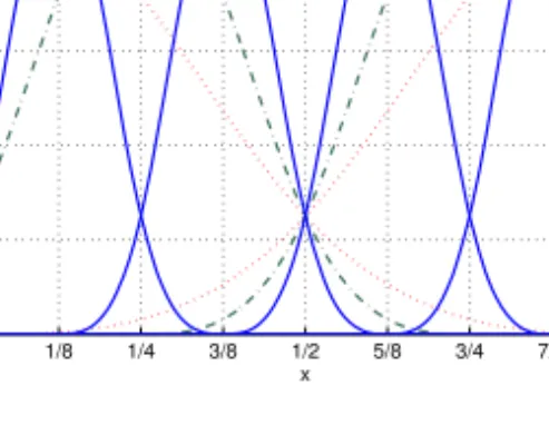
Figure 1. Hierarchical B-splines (ψi()(x)) of order 3. Level 0 (- - -), level 1 (···), level 2 (-·-) and level 3 (—) basis functions.
wherec()i andφi()(x)are thei-th vectorial coefficient and the related basis function at level, the latter is an element ofΦ(x)in (2), andm(N) is the number of basis functions at levelin anN-D sparse grid, respectively.
Linear (“hat”) basis functionsψi()(x)are commonly used with sparse grids. In the present work,hierarchicalB-spline basis functions are applied, and similarly to [8], 3rd order B-splines have been chosen. This choice ensures the continuity of the 2nd order derivatives of interpolant (3). The 3rd ordercardinalB-spline is defined in the interval 0≤x≤4 and it is expressed as
b(3)(x) =
⎧⎪
⎪⎨
⎪⎪
⎩
1/4x3, 0≤x<1;
−3/4x3+3x2−3x+1, 1≤x<2;
3/4x3−6x2+15x−11,2≤x<3;
−1/4x3+3x2−12x+16,3≤x≤4.
(4)
In our implementation, the level 0 basis function is chosen as constant (ψ1(1)(x) =1) and all other hierarchical basis functions (≥1) are derived from a cardinal B-spline (4) via an affine transformation of the input variable, as illustrated in Fig. 1.
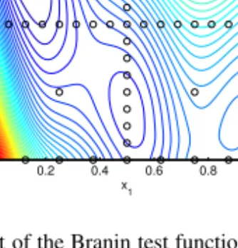
To determine the coefficientsc()i in (3), the equality ˆf(xk) =f(xk)is enforced atn number of control points (xk,k=1,2,...,n). These points are chosen as the center points of the corresponding basis functions (i.e., whereφi()(x) =1 hold, for all≥1, and by definition, it is1/2[1,1,...,1]forφ1(0)(x)). The number of control points is thus equal to the cardinality of the sparse basis (2), and the location of the set of these control points (nodes) forms the so-calledsparse grid. In 2-D, the distribution of the sparse grid nodes is illustrated in Fig. 2, along with the contour lines of the sparse grid interpolant of the well-known Branin test function [9].
The sparse grid interpolation can cope with the curse-of-dimensionality in the fol- lowing sense. The number of grid nodesn in a sparse grid with depthd in dimension Nis in the orderO{K(logK)N−1}, whereK=2d+1 being the number of hierarchical basis functions per dimension. However, the increase ofn is much faster when a clas- sical full grid is used, hereinO{KN}applies [4]. The numerical example presented in Sec. 4 involvesN=4 dimensions, for which the node numbers of sparse and full grids
x1 x2
Spline basis, depth = 3
0 0.2 0.4 0.6 0.8 1
0 0.2 0.4 0.6 0.8 1
Figure 2. Contour lines of the interpolant of the Branin test function by means of a depth=3 sparse grid with hierarchical B-spline basis functions, along with the grid nodes.
Table 1. Node numbers of sparse and full grids inN=4 dimension, in function of the depthd.
d 0 1 2 3 4 5 6
n(sparse) 1 9 41 137 401 1105 2929
n(full) 1 81 625 6561 83521 1185921 17850625
are compared in Table 1 as an illustration of the gain benefited from sparse grids. In spite of the large reduction of node numbers, the interpolation accuracy of sparse grids is only slightly deteriorated compared to full grids, as detailed in [4].
3. Inversion using the sparse grid surrogate model
Once the sparse grid surrogate model (3) is available, and hierarchical B-splines are used as basis functions therein, one can solve the inverse problem by means of opti- mizing a misfit function, as it follows. Let us assume that the outputy of the numeri- cal simulationf(x)(as already mentioned in Sec. 2) is a real row vector ofMelements:
y= [y1,y2,...,yM]. In the case of complex output (e.g., complex impedance variation in EC-NdT), one can always introduce the real output vector asy:= [Re{y},Im{y}]. The measured data vector is denoted by ˜y. Let us define the quadratic misfit function as the squared norm of the discrepancy between simulated and measured data:
u(x) =y˜−y2≡[y˜−y][˜y−y]T (5) The regularized inverse problem then consists in solving the constrained optimization problem
x=arg min
x∈[0,1]Nu(x) (6)
that yields the solution x. In order to reduce the computational burden, one approxi- matesy=f(x)by ˆy=ˆf(x), and the approximate misfit function ˆu(x) =y˜−yˆ2is to be minimized according to (6). Since ˆf(x)is based on a sparse grid interpolation with hierarchical B-spline basis functions, its gradient
∇ˆf(x) =
⎡
⎢⎣
∂yˆ1/∂x1 ∂yˆ2/∂x1 ···∂yˆM/∂x1
... . .. ...
∂yˆ1/∂xN∂yˆ2/∂xN ···∂yˆM/∂xN
⎤
⎥⎦ (7)
can be easily expressed in closed form based on (3). Therefore, one can also write the gradient of the quadratic approximate misfit function in closed form (see, e.g., [10]) as
∇u(ˆ x) =2[˜y−ˆf(x)][∇ˆf(x)]T. (8) This gradient (8) can be used in the gradient-based solution of the optimization prob- lem (6). In order that one can choose among the large variety of classical unconstrained optimization algorithms, the constrained problem (6) has to be re-formulated by using some nonlinear transformation of the optimization variable x. Herein a new variable ξ = [ξ1,ξ2,...,ξN]is introduced such that
xi= (arctanξi)/π+1/2, xi∈[0,1], ξi∈(−∞,∞), i=1,2,...,N, (9) and the optimization is performed with respect toξ in an unconstrained domain:
ξ=arg min
ξ∈RN u(x(ξ)). (10)
The gradient-based local optimization strategies unfortunately suffer from the pos- sibility of stalling in a local minimum and thus miss the global minimum. This risk is reduced when one runs the algorithm with different initial guesses. However, this was not the case in the numerical example which is presented in the next section.
4. Numerical example 4.1. Configuration
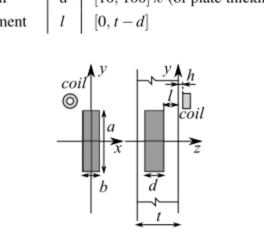
Let us consider the eddy-current testing arrangement shown in Fig. 3. A homogeneous, non-ferromagnetic plate is considered as specimen. The conductivity isσ=106S/m and the thickness ist=1.55 mm. The other dimensions of the plate are assumed to be infinite.
The coil is an air-cored probe (inner and outer diameters: 2 mm and 3.25 mm; height:
2 mm; no. of turns: 328; lift-offh: 0.303 mm), driven with a time-harmonic current with frequency of 300 kHz. The variation of the coil impedance is observed at regularly spaced coil positions:
xc={−15 : 1 : 15}mm and yc={−5 : 1 : 5}mm, (11) that is, 31×11=341 complex impedance variations are available in the surface scan.
A rectangular-shaped defect (with zero conductivity) is present within the plate, with sides parallel to thex,yandzaxes; the defect is centered on the origin of thexyplane. The bounds given in Table 2 apply for the 4 geometrical parameters of the defect. The input domain is non-rectangular but narrowed by a linear inequality constrain fordandl. This
Table 2. Parameter ranges in the single narrow crack example.
parameter range length a [4,22]mm width b [0.001,0.3]mm
depth d [10,100]% (of plate thickness) ligament l [0,t−d]
l
d a
b coil
x y
z
t y h
coil
Figure 3.Sketch of the configuration.
is taken into account when transforming the input domain to the[0,1]N hypercube, on which the sparse grid and inversion algorithms are performed, as already seen in Sec. 2.
The electromagnetic simulation is based on an integral equation formulation, imple- mented in the CIVA software [11].
4.2. Test of the forward interpolation
The interpolation error is defined asε(x) =fˆ(x)−f(x)at each pointx. The overall interpolation performance is characterized by the maximal and root mean-squared (rms) interpolation error, both are approximated based on a finite number of test samplesxj (j=1,2,...,J):
εmax=max
j ε(xj), εrms= 1
J
∑
j
ε(xj)2 (12)
In this numerical test, 4000 random test samples are used. In order to facilitate the in- terpretation of the error, the normalized (dimensionless) interpolation error is presented, with a normalizing factor that is chosen as max
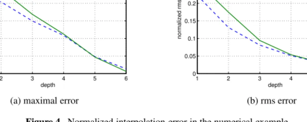
j f(xj). The change of the normalized error with respect to the depth of the sparse grid interpolation is shown in Fig. 4. For reference, linear basis functions [5] have also been used. In terms of interpolation accu- racy, the linear basis slightly outperforms the B-splines. Yet, the B-splines are better in optimization-based inversion schemes, as shown in the next section.
4.3. Test of the inversion algorithm
As summarized in Table 3, the output signal associated with two randomly chosen de- fects (denoted as “true”) has been calculated. The inversion procedure detailed in Sec. 3 resulted in the reconstructed parameters denoted as “grad”. For comparison, a similar optimization-based inversion has been performed using the sparse grid with linear basis functions (the same as presented in the previous section). Due to the lack of continuous
1 2 3 4 5 6 0.2
0.3 0.4 0.5 0.6 0.7 0.8 0.9
depth
normalized max error
linear spline
(a) maximal error
1 2 3 4 5 6
0 0.05 0.1 0.15 0.2 0.25 0.3 0.35
depth
normalized rms error
linear spline
(b) rms error Figure 4. Normalized interpolation error in the numerical example.
Table 3. Results of the inversion in the 1st (left) and 2nd (right) test cases. The “true” parameters correspond to the defect to be reconstructed, and the gradient-based (“grad”) and simplex optimisation-based (“direct”) inversion methods yielded the parameters as given in the tables. Depth=6 sparse grid is used in all cases.
a b d l
true 16.04 0.290 0.258 0.413 grad 16.30 0.012 0.474 0.324 direct 20.42 0.118 0.348 0.389
a b d l
true 15.10 0.157 0.525 0.942 grad 14.96 0.188 0.507 0.957 direct 16.20 0.137 0.478 0.850
gradient of the interpolant, a simplex optimization (referred to as “direct”) method has been applied with the linear basis. According to Table 3, both approaches found reliable solutions, except for parameterb, which is the width of the defect and it is well-known to have only a weak influence on the impedance change. This measurement setup thus has limited capacity in reconstructingb.
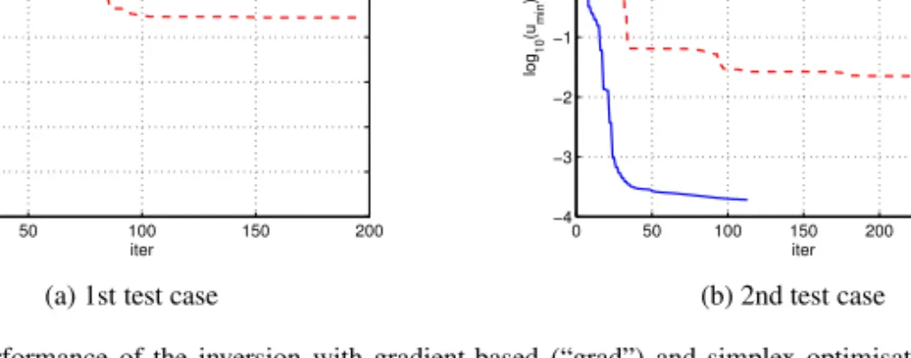
The main advantage of the B-spline based scheme becomes clear when looking at the evolution of the iterative optimization routines in Fig. 5. In both examples, the gradient method converged much faster to a better local minimum than the simplex method.
Implementation has been made in Matlab, with the functionsfminunc(a quasi- Newton method) andfminsearch(a simplex method for direct search).
5. Conclusion
The use of B-spline basis functions for interpolation on sparse grids has been found to be an efficient tool when performing optimization-based inversion using the sparse grid surrogate model. The gradient of the approximate misfit function is continuous, giving rise to gradient methods. Spare gridsper sehave previously proven a good performance in NdT inversion; and the present contribution is an extension of this solid framework.
Future work will include the expression the Hessian of the misfit function to use second order optimization methods. Furthermore, one will study the case when the gra- dient of the forward modelfis available at hand (e.g., via the adjoint problem), and it can be used to fit the surrogate model not only tofbut to∇fas well. Considerations on the adaptive generation of the sparse grid in combination with B-spline basis functions will also be taken.
0 50 100 150 200
−3
−2.5
−2
−1.5
−1
−0.5 0 0.5 1
iter log10(umin)
grad direct
(a) 1st test case
0 50 100 150 200 250 300
−4
−3
−2
−1 0 1 2
iter log10(umin)
grad direct
(b) 2nd test case
Figure 5. Performance of the inversion with gradient-based (“grad”) and simplex optimisation-based (“di- rect”) inversion methods: minimum misfit function found with respect to iteration number.
Acknowledgment
The work was created in commission of the National University of Public Service under the priority project K ¨OFOP-2.1.2-VEKOP-15-2016-00001 titled “Public Service Devel- opment Establishing Good Governance” in the Bay Zolt´an Ludovika Workshop. Further support was provided by the Hungarian Scientific Research Fund under grant K-111987 and by the J´anos Bolyai Research Scholarship of the Hungarian Academy of Sciences.
References
[1] G. Franceschini, M. Lambert, and D. Lesselier, “Adaptive database for eddy-current testing of metal tube,” inProceedings of the 8th International Symposium on Electric and Magnetic Fields (EMF 2009), Mondovi, Italie, May 2009, (on CDROM).
[2] S. Gyim ´othy, “Optimal sampling for fast eddy current testing inversion by utilising sensitivity data,”IET Science, Measurement & Technology, vol. 9, no. 3, pp. 235 – 240, 2015.
[3] R. Douvenot, M. Lambert, and D. Lesselier, “Adaptive metamodels for crack characterization in eddy- current testing,”IEEE Transactions on Magnetics, vol. 47, no. 4, pp. 746–755, 2011.
[4] H.-J. Bungartz and M. Griebel, “Sparse grids,”Acta Numerica, vol. 13, pp. 147–269, 2004.
[5] S. Bilicz, “Sparse grid surrogate models for electromagnetic problems with many parameters,”IEEE Transactions on Magnetics, vol. 52, no. 3, pp. 1–4, 2016.
[6] C. Cai, S. Bilicz, T. Rodet, M. Lambert, and D. Lesselier, “Metamodel-based nested sampling for model selection in eddy-current testing,”IEEE Transactions on Magnetics, vol. 53, no. 4, pp. 1–8, 2017.
[7] L. Zhou, H. A. Sabbagh, E. H. Sabbagh, R. K. Murphy, W. Bernacchi, J. C. Aldrin, D. Forsyth, and E. Lindgren, “Eddy-current NDE inverse problem with sparse grid algorithm,”AIP Conference Pro- ceedings, vol. 1706, no. 1, p. 090016, 2016.
[8] J. Valentin and D. Pfl ¨uger,Sparse Grids and Applications - Stuttgart 2014. Springer International Publishing Switzerland, 2016, ch. Hierarchical Gradient-Based Optimization with B-Splines on Sparse Grids, pp. 315–336.
[9] A. Forrester, A. Sobester, and A. Keane,Engineering design via surrogate modelling: a practical guide.
Wiley, 2008.
[10] A. Tarantola,Inverse Problem Theory and Model Parameter Estimation. SIAM, 2005.
[11] CIVA: A state-of-art simulation software in ndt. [Online]. Available: http://www.extende.com