Sensitivity Analysis Using a Sparse Grid Surrogate Model in Electromagnetic NDE

Sensitivity Analysis Using a Sparse Grid Surrogate Model in Electromagnetic NDE

Arnold BINGLER¹and S´andor BILICZ² Budapest University of Technology and Economics

Abstract.The global sensitivity analysis of electromagnetic nondestructive evalu- ation (NDE) by means of Sobol’ indices are considered in this work. To reduce the computational burden, a sparse grid surrogate model is used. The latter can simply replace the true simulator to some extent, but it can also be used to numerically evaluate the integrals defining the Sobol’ indices. In most of the NDE setups, the output is not a scalar quantity but functional data (e.g., a surface scan); a method is presented to take this into account. The sparse grid based sensitivity analysis is compared to classical techniques via examples drawn from electromagnetic NDE.

Keywords.sensitivity analysis, Sobol’ index, sparse grid

1. Introduction

To characterize the uncertainty of the output of a simulation model due to its uncertain input parameters, Sobol’ indices are commonly used. However, the calculation of the Sobol’ indices can be computationally demanding, especially in the case when a heavy simulator is considered and/or the number of input parameters is high. The application of surrogate models provides a way to reduce this computational burden. Polynomial Chaos Expansion (PCE) supplies an efficient, low-cost technique to compute the Sobol’

indices. Recently, the use of sparse grids (SGs) in electromagnetic nondestructive eval- uation (ENDE) has been proposed [1]. SG can be used both as an approximation of the model (e.g., for Monte Carlo method) and as a numerical quadrature to evaluate inte- grals involved in the calculation of Sobol’ indices. The surrogate model-based sensitivity analysis in the context of ENDE is considered, e.g., in [2]. The present work aims at (i) comparing different surrogate model based approaches of Sobol’ index calculation for ENDE problems and (ii) extending the formulations to the case when the output consists of functional data, being typical in ENDE (e.g., surface scan of an eddy-current probe).

1E-mail: arni38@sch.bme.hu

2Corresponding Author: S´andor Bilicz; E-mail: bilicz@evt.bme.hu

© 2018 The authors and IOS Press.

This article is published online with Open Access by IOS Press and distributed under the terms of the Creative Commons Attribution Non-Commercial License 4.0 (CC BY-NC 4.0).

doi:10.3233/978-1-61499-836-5-152

2. Sensitivity Analysis

In this section a brief overview is given on the purpose of the sensitivity analysis, par- ticularly with respect to the method of Sobol’ indices as well as the possibilities of its numerical calculation.

Suppose that we have a mathematical modely=f(xxx)as a multivariate, square inte- grable function over a domain defined by a set of independent variables,xxx= (x1,...,xn). In general the aim of sensitivity analysis is the quantification of how the uncertainty of the model output is affected by the uncertain input parameters. Theblack-boxapproach is commonly used, i.e., one relies only on certain number of input samples and the cor- responding output ones. This approach provides the flexibility of applications in wide range of industrial and scientific fields.

2.1. Sobol’ indices

The technique of Sobol’ indices is a variance-based sensitivity analysis method. After its introduction in [3], by now it has become a widely used approach in several fields. A detailed presentation is given in, e.g., [4]. A brief summary is given below, such that the novelty of the present work can be clearly pointed out.

Without the loss of generality we can assume that all input variables are uniformly and independently distributed in the unit hypercubeDxxx= [0,1]ⁿ. The key idea is to de- composef(xxx)into the sum of subfunctions of increasing dimension, such that

f(xxx) =f0+

∑

i=1

fi(xi) +

∑

1≤i<j≤n

fi j(xi,xj) +···+f_1,2,...,n(x1,x2,...,xn) (1)

with f0being the expected value of f(xxx)and the integral of the subfunctions with re- spect to any of their arguments is zero, i.e., the subfunctions are pairwise orthogonal.

This Sobol-decomposition is shown to be uniquely exist in [3], and the subfunctions are defined in a recursive manner:

f0=

Dxxx

f(xxx)dxxx (2a)

fi(xi) = ¹

0 ··· ¹

0

f(xxx)dxxx∼i−f0 (2b)

fi j(xi,xj) = ¹

0 ··· ¹

0 f(xxx)dxxx_∼i,j−f0−fi(xi)−fj(xj) (2c) wherex_∼iis a set withoutxi. In addition the variance of f(xxx)can be partitioned into the sum of sub-variances:

D=

∑

vvv⊆xxx\{0}

Dvvv, (3)

with Dvvv denoting the variance of the subfunction described by a group of variables vvv= (xi₁,xi₂,...,xis). Each sub-variance can be considered as the contribution of a group

of variables to the total variance. The measure of their importance, namely the Sobol’

indices thus can be defined as

Svvv=Dvvv

D. (4)

The sum of all possible indices is 1, providing us a simple interpretation of their meaning.

Groups consist of only one variable yield the 1st order indices. The 2nd order ones mean the effects caused by the interaction of two parameters without their 1st order effects;

higher order indices can be analogously defined. Traditionally, the 1st order indices are estimated by Monte Carlo formulas:

fˆ0=

∑

k=1

f(xxx^(k)) (5a)

Dˆ =

∑

k=1

f(xxx^(k))²−fˆ0

2 (5b)

Dˆi=

∑

k=1

f(x^(k)_i ,xxx^(k)_∼i)f(x^(k)_i ,xxx^(k)_∼i)−fˆ0

2 (5c)

wherexxx^(k) is thek-th representation of theM samples andxxx^(k)_∼i denotes a sample inde- pendent fromxxx^(k)_∼i

2.2. Extension of Sobol’ indices

In the original framework of Sobol’ indices, the output is a scalar function and the vari- ables have to be independent. In certain cases this can be sufficient (e.g., scalar-output indices for POD studies), however, several NDE related applications cannot be directly treated due to these limitations. For example, vector output functions occur when a sur- face scan of impedance variation is considered or geometric constraints apply for the defect parameters, making them dependent on each other. Therefore, the original defini- tion needs to be extended and generalized regarding the above cases, which is the main contribution of this work.

2.2.1. Multiple output functions

Supposing we have a multiple output functionF(xxx) =

F1(xxx),F2(xxx),...,FP(xxx)

, a natural extension of Sobol’ indices is taking the average of the previously calculated indices of the component functions, i.e.,

S^avg_i =1 P

∑

S⁽_Fⁱ⁾

j. (6)

This method has its drawback by not taking into account the vectorial nature of the output and the correlation between the component functions. A more suitable solution requires the definition of global indices to the entire functional output. A method with

this consideration has recently been introduced in [5]. Hereby we give another, simpler approach to extend the 1st order indices, relying on an equivalent stochastic definition:

Si=Varxi[Exxx_∼i[f(xxx)|xi]]

Var[f(xxx)]. (7)

In 1 dimension (1-D), variance can be considered as the expected value of a squared error function, defined by the deviation of f(xxx)from its own expected value. InN-D, variance can be defined analogously with the error being a vector and the 2-norm is used as a metric of distance instead of absolute value:

D^vec=E h²2

=E

F(xxx)−F₀²2

, (8)

whereF₀denotes the vectorial expected value of F(xxx). This leads us the definition of vectorial Sobol’ indices:

S^vec_i =Varxi[Exxx_∼i[F(xxx)|xi]]

Var[F(xxx)] =D^vec_i

D^vec. (9)

Monte Carlo estimators are also extended to vectorial outputs as Fˆ₀= 1

M

∑

F(xxx^(k)) (10a)

Dˆ^vec= 1 M

∑

k=1F(xxx^(k))²2− Fˆ₀²2 (10b) Dˆ^vec_i = 1

M

∑

F(x^(k)_i ,xxx^(k)_∼i)•F(x^(k)_i ,xxx_∼i^(k))− Fˆ₀²2 (10c) with•denoting the scalar multiplication. Though the squared Euclidean norm fits well for our purpose, we note that this choice is not obvious. In the case of a sparse output signal—which is typical, e.g., when a temporal echo is recorded in an ultrasonic testing method—other norms (such as the maximum norm) might be preferred. One may also consider an appropriate pre-processing of the signal before using the Euclidean norm.

2.2.2. Dependent variables

A method of sensitivity analysis over non-rectangular domain has recently been studied in [6]. Herein we introduce a method based on theRosenblatt transform(RT) proposed in [7]. Let us denote withxxx^∗a permutation ofxxxand withFi(x^∗_i|vvv)being the conditional cumulative distribution function ofx^∗_i with respect to a subsetvvv⊆xxx^∗_∼i. It is known that the joint probability density function ofxxx^∗can be decomposed as follows:

p(xxx^∗) =p(x^∗1)p(x^∗2|x^∗1)p(x^∗3|x^∗1,x^∗2)...p(x^∗n|xxx^∗_∼n). (11) Based on (11), Rosenblatt transform provides a bijective mapping to the unit hypercube U∼[0,1]ⁿ:

F1(x^∗1) =u1, F2(x^∗2|x^∗1) =u2, ..., Fn(x^∗n|xxx^∗_∼n) =un. (12)

There aren! different transforms due to the permutations ofxxx, however, the results of interest narrow into two special cases concerningxi. In the case ofxi=x^∗₁, the transform is performed via the marginal distribution function ofxi, hence contains the effect from the constraints as well, while in the case ofxi=x^∗_n, these effects are excluded due to the fact thatFiis conditional to all other variables. Therefore the authors in [7] call the 1st order Sobol’ indices ofxigained from these special transforms as full and individual in- dices, respectively. These indices characterize the uncertainty contribution of dependent variables.

3. Surrogate Models

Performing sensitivity analysis usually requires the modelling of the examined configu- ration in many settings of the input parameters in order to get the proper number of sam- ples to Monte Carlo simulation. At each sample the electromagnetic model is evaluated (e.g., finite-element model, integral equation model), which might lead to a very long simulation. To reduce the computational burden due to the “curse of dimensionality”, surrogate models are used as low-cost approximations of the true simulator, usually con- structed as a linear combination of a set of orthonormal multivariate basis functions. In general a set of orthonormal univariate basis functionsΨΨΨ(x) ={Ψ1(x),Ψ2(x),... ,Ψl(x)}

is created in the first step, then the multivariate ones are built as their tensor product:

ΦΦΦ(xxx) =ΨΨΨ(x1)⊗ΨΨΨ(x2)⊗ ··· ⊗ΨΨΨ(xn). (13) This set can be truncated to a set of lower cardinality, yielding the surrogate model as

f(xxx)≈ fˆ(xxx) =

∑

i∈AαiΦi(xxx) (14)

with A being an index set. Basically, the differences between the numerous data-fit models are the strategy behind the construction of the univariate basis, the truncation scheme and the estimation of the coefficients. Herein two commonly used methods are briefly summarized: the Polynomial Chaos Expansion (PCE) and the Sparse Grid (SG) interpolation.

Polynomial Chaos Expansion. The PCE provides approximation in a stochastic frame- work of f(xxx)by choosing the basis functions to be orthonormal with respect to the joint probability density function ofxxx, e.g., Legendre-polynomials for variables uniformly dis- tributed in]−1,1[, Hermite-polynomials for Gaussian distributions, etc. [4] The trunca- tion might be performed by giving a limit on the highest occurring polynomial degree.

The coefficients are traditionally calculated from random input and output samples by the ordinary least-squares method:

αααˆ ≈arg minE

⎡

⎣

f(xxx)−

∑

i∈AαiΦi(xxx) 2⎤

⎦. (15)

There is strong link between Sobol’ decomposition and PCE due to the uniqueness of the former one and the orthogonality of the basis functions. The variance of f(xxx) is

a2

a1

t

x

(a) MFL example.

x y

z y

d

a

h

t l σ

(b) EC-NdT example.

Figure 1. Sketch of the configurations. MFL parameters:a1,2∈[0.6,1.2]mm andd1,2∈[0.2,1.6]mm. EC-NdT parameters:t= (1.25±0.01)mm,σ= (1±0.01)MS/m,h= (0.5±0.05)mm,a∈[2,10]mm,d∈[0.125,1]mm andl∈[0.125,1.125]mm.

partitioned into the sum of the square of the coefficients, providing a convenient way to evaluate the sub-variances and the Sobol’ indices.

Sparse grid interpolation. SG interpolation (detailed in [1], [8]) is based on the eval- uation of the original model at specific points, calling them the supporting nodes. The basis functions have a hierarchical structure of level-by-level, each of them belongs to a supporting nodex⁽ⁱ⁾_l . Their tensor product results in a multivariate basis that can be truncated by, e.g., a linear constraint on the sum of the levels:∑ⁿi=1li=l. In the case of linear (“hat”) basis functions, the interpolant at depthdequals to the sum of interpolant from the previous depth and the linear combination of the multivariate functions at level d:

fˆ(xxx)≈fˆd(xxx) =fˆd−1(xxx) +^m

∑

i=1

Φ⁽ⁱ⁾_d (xxx)

f(xxx⁽ⁱ⁾_d )−fˆd−1(xxx⁽ⁱ⁾_d )

v⁽_dⁱ⁾

(16)

with ˆf0(xxx) =Φ⁽¹⁾₀ (xxx)f(xxx⁽¹⁾₀ )andxxx⁽ⁱ⁾_d denoting the vector of 1-D nodes belonging to the 1-D functions ofΦ⁽ⁱ⁾_d . The coefficientsv⁽ⁱ⁾_d are equal to the difference between f(xxx)and fˆ_d−1(xxx)at the nodesxxx⁽ⁱ⁾_d . The SG provides a surrogate model to generate Monte Carlo samples, however, it can be used as numerical quadrature to directly evaluate the integrals in (2), similarly to PCE [9].

4. Numerical examples

Magnetic Flux Leakage NdT (4-parameter model). A ferromagnetic plate of thickness t=2 mm andμr=100 is corrupted by grooves infinitely perpendicular to thex-axis.

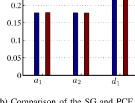
The grooves are described by 4 parameter-cubic splines, with parameters uniformly dis- tributed as given in the caption of Fig. 1. A homogeneousHx0=1 A/m magnetic field is imposed in thexdirection. The distortion field (ΔHx) is measured at 51 equidistant points on the top of the surface. The depths of the grooves were found to be more important pa- rameters compared to their widths (Fig. 2a). Good correlation between the vectorial and

0 0.05 0.1 0.15 0.2 0.25 0.3 0.35

a1 a2 d1 d2

vectorial average

(a) 1st order vectorial and average Sobol’ indices.

0 0.05 0.1 0.15 0.2 0.25 0.3 0.35

a1 a2 d1 d2

SG PCE

(b) Comparison of the SG and PCE based direct ap- proaches by the average indices.

Figure 2. Results of the MFL example.

0 0.1 0.2 0.3 0.4 0.5 0.6 0.7

d l a

full individual

(a) Full and individual 1st order indices of the defect parameters whileh,t,σare kept at their mean value.

10⁵ 10⁶

−0.2 0 0.2 0.4 0.6 0.8 1 1.2

No. of samples in the MC method h

t σ

(b) Convergence of the setup parameters whiled,l,a are kept at their mean value.

Figure 3. Results of the EC-NdT example.

averaging method can be observed. Direct methods equally resulted in the same outcome as MC-based calculation (Fig. 2b).

Eddy-Current NdT (3+3 parameter model). An infinite, non-ferromagnetic, conductive plate with a thicknesstand conductivityσis investigated as shown in Fig. 1b. The plate includes an ideal crack described by 3 parameters from which d andl are dependent ones due to thed+l≤t constraint. A coil with time-harmonic excitation of 150 kHz is scanning over the surface at a lift-offh. The change of its impedance is measured at 297 test points of the grid(x,y)∈ {−2 : 0.5 : 2} × {−8 : 0.5 : 8}mm. A single model evaluation needs 15 seconds by the integral equation simulation [10], thus a SG model was built to reduce computation time. A cross-validation was also performed to ensure its accuracy; RMS-error of 4 % with depth=5, below 0.1 % with depth=7 was achieved. Due to the complex nature of the output vector, it had to be transformed to a 594-element real- valued vector asF(xxx)⇒[Re{F(xxx)}; Im{F(xxx)}]. The sensitivity analysis was performed by dividing the parameters into two groups: defect parameters (a,d,l) and parameters of the measurement setup (h,t,σ^).

The depth of the crack was repeatedly found to be the most important defect pa- rameter as both its individual and full index are the highest ones (Fig. 3a). The lift-off hexceeds out of the setup parameters, while the conductivity has almost no effect. The convergence study confirmed that the number of required samples need to be close to the order of millions (Fig. 3b).

5. Summary

The proposed extension of the Sobol’ indices is found to be an appropriate technique to characterize the effect of uncertain parameters on a complete line/surface scan. To some extent, dependent uncertain input parameters can also be treated. The presented tools are shown to apply well to various NdT examples, the conclusions coincide with the physical expectations. Future work will include further reduction of the required sample number by means of PCE coefficients.

Acknowledgment

The work was created in commission of the National University of Public Service under the priority project K ¨OFOP-2.1.2-VEKOP-15-2016-00001 titled “Public Service Devel- opment Establishing Good Governance” in the Bay Zolt´an Ludovika Workshop. Further support was provided by the Hungarian Scientific Research Fund under grant K-111987 and by the J´anos Bolyai Research Scholarship of the Hungarian Academy of Sciences.

References

[1] S. Bilicz, “Sparse grid surrogate models for electromagnetic problems with many parameters,”IEEE Transactions on Magnetics, vol. 52, no. 3, pp. 1–4, 2016.

[2] R. Miorelli, X. Artusi, A. B. Abdessalem, and C. Reboud, “Database generation and exploitation for efficient and intensive simulation studies,” inAIP Conference Proceedings 1706, 2016.

[3] I. M. Sobol’, “Sensitivity estimates for nonlinear mathematical models,”Mathematical Modelling and Computational Experiments, vol. 1, no. 4, pp. 407–414, 1993.

[4] B. Sudret, “Global sensitivity analysis using polynomial chaos expansions,”Reliability Engineering &

System Safety, vol. 93, no. 7, pp. 964–979, 2008.

[5] F. Gamboa and A. L. Alexandre Janon, Thierry Klein, “Sensitivity indices for multivariate outputs,”

Comptes Rendus Mathematique, vol. 351, no. 7-8, pp. 307–310, 2013.

[6] S. Kucherenko, O. Klymenko, and N. Shah, “Sobol indices for problems defined in non-rectangular domains,”Reliability Engineering & System Safety, vol. 167, pp. 218–231, 2017.

[7] T. A. Mara, S. Tarantola, and P. Annoni, “Non-parametric methods for global sensitivity analysis of model output with dependent inputs,”Environmental Modelling and Software, Elsevier, vol. 72, pp.

173–183, 2015.

[8] H.-J. Bungartz and M. Griebel, “Sparse grids,”Acta Numerica, vol. 13, pp. 147–269, 2004.

[9] G. T. Buzzard, “Global sensitivity analysis using sparse grid interpolation and polynomial chaos,”Reli- ability Engineering & System Safety, vol. 107, pp. 82–89, 2012.

[10] J. P´av´o and D. Lesselier, “Calculation of eddy current testing probe signal with global approximation,”

IEEE Transactions on Magnetics, vol. 42, no. 4, pp. 1419–1422, 2006.