(2010) pp. 177–189
http://ami.ektf.hu
CTH B-spline curves and its applications ∗
Jin Xie
ab, Jieqing Tan
ac, Shengfeng Li
adaSchool of Computer and Information, Hefei University of Technology, Hefei, China
bDepartment of Mathematics and Physics, Hefei University, Hefei, China
cSchool of Mathematics, Hefei University of Technology, Hefei, China
dDepartment of Mathematics and Physics, Bengbu College, Bengbu, China
Submitted 21 April 2010; Accepted 26 August 2010
Abstract
A method of generating cubic blending spline curves based on weighted trigonometric and hyperbolic polynomial is presented in this paper. The curves inherit nearly all properties of cubic B-splines and enjoy some other advantageous properties for modeling. They can represent some conics and some transcendental curves exactly. Here weight coefficients are also shape parameters, which are called weight parameters. The interval [0,1] of weight parameter values can be extended to[(ee−1)−1)22
−π,(e−1)e−1)2π22π−82 e]. Not only can the shape of the curves be adjusted globally or locally, but also the type of some segments of a blending curve can be switched by taking different values of the weight parameters. Without solving system of equations and letting certain weight parameter be (2(e−1)2(2−π)
e−1)2−2π, the curves can interpolate corresponding control points directly.
Keywords: cubic uniform B-spline, CTH B-spline, weight parameter, local and global interpolation, local and global adjustment, transcendental curve MSC:68U05
1. Introduction
B-spline curves and surfaces are well known geometric modeling tools in Computer Aided Geometric Design (CAGD). Due to their several limitations in practical ap- plications[1], several new forms of curve and surface schemes have been proposed
∗Reaserch supported by the National Nature Science Foundation of China (No.61070227), the Doctoral Program Foundation of Ministry of Education of China (No. 20070359014) and the Key Project Foundation of Scientific Research for Hefei university (No.11KY02ZD).
177
for geometric modeling in CAGD[2-12]. C-curves are introduced in [2,3] by us- ing the basis {1, t, cost, sint} instead of{1, t, t2, t3} in cubic spline curves, which can represent some transcendental curves such as the ellipse, the helix and the cycloid. Further properties of C-curves have been studied in [4]. Hoffmann et al.
[5] investigated a geometric interpretation of the change of parameter αfor C-B- spline curves. Similarly, using the hyperbolic basis {1, t, cosht, sinht} instead of {1, t, t2, t3}in cubic uniform B-splines, one can construct a curve family too. This has been studied as exponential B-splines [6,7,8]. Just for convenience, we call them HB-splines. Koch and Lyche[6] presented a kind of exponential splines in tension in the space spanned by {1, t, cosht, sinht}. Lü et al.[7] gave the explicit expressions for uniform splines. Li and Wang[8] generalized the curves and surfaces of exponential forms to algebraic hyperbolic spline forms of any degree, which can represent exactly some remarkable curves and surfaces such as the hyperbola, the catenary, the hyperbolic spiral and the hyperbolic paraboloid.
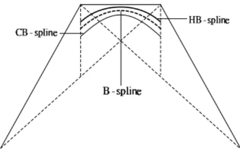
CB-splines and HB-splines are the same in structure and their shapes are ad- justable. However, after comparing CB-splines and HB-splines, we found that a CB-spline is located on one side of the B-spline, and the HB-spline is located on the other side of the B-spline, see Figure 1. Therefore, one thinks whether the two different curves can be unified. If we can unify them, then the new curve will have more plentiful modeling power. In order to construct more flexible curves for the surface modeling, Zhang et al. [9,10] proposed a curve family, named FB- spline, that is the unification of CB-spline and HB-spline. However, the formulas for the FB-splines were rather complicated. Hoffmann et al. [11] introduced prac- tical shape modification algorithms of FB-spline curves and the geometrical effects of the alteration of shape parameters, which are essential from the users’ point of view. Wang and Fang[12] unified and extended three types of splines by a new kind of spline (UE-spline for short) defined over the space {cosωt, sinωt,1, t, ..., tl, ...}, where the type of a curve can be switched by a frequency sequence{ωi}.
Figure 1: CB-spline and HB-spline are located on the different sides of B-spline In this paper, we present a set of new bases by unifying the trigonometric basis and the hyperbolic basis using weight method, which inherits the most properties of cubic uniform B-spline bases. Based on those bases, we introduce a new spline curve, named CTH B-spline curve. This approach has the following features:
• The introduced curves can cross the B-splines and reach the both sides of cubic B-splines.
• The shape of the curves can be adjusted globally or locally.
• Without solving system of equations and letting weight parameters be(e− 1)2(2−π)/(2(e−1)2−2π), the curves can interpolate certain control points directly.
• With the weight parameters and control points chosen properly, the CTH B- spline curves can be used to represent some conics and transcendental curves.
• The type of the curves can be switched by letting weight parametersλi = 0 or 1 easily. And, a blending curve can be composed of different type curve segments.
The rest of this paper is organized as follows. In Section 2, the basis functions unified by the trigonometric basis and the hyperbolic basis using weight method are established and the properties of the basis functions are shown. In Section 3, the CTH B-spline curves are given and some properties are discussed. It is pointed out in Section 4 that some transcendental curves can be represented precisely with the CTH B-spline curves and the applications of the curves are shown in Section 5. Finally, we conclude the paper in Section 6.
2. The construction of CTH B-spline basis functions
In order to construct CTH B-spline basis functions, we give two classes of basis functions as follows.
Definition 2.1. The following functions,
T0,3(t) =1−2t−1πcosπ2t,
T1,3(t) =2t+π2cosπ2t−π1sinπ2t, T2,3(t) =1−2t+π2sinπ2t−1πcosπ2t,
T3,3(t) = t2−1πsinπ2t, are called CT B-spline basis functions.
Remark 2.2. The CT B-spline basis functions are the CB-spline basis functions withα=π/2, see[3].
Definition 2.3. The following functions,
H0,3(t) =−(e−e1)2(1−t) +(e−e1)2sinh(1−t),
H1,3(t) =−(e−e1)2 +1+e+e(e−1)22(1−t) +2(ee+1−1)cosh(1−t) +1+4e+e(e−1)2π2sinh(1−t),
H2,3(t) =−(e−e1)2 +1+e+e(e−1)22t+2(ee+1−1)cosht+1+4e+e(e−1)2π2sinht, H3,3(t) =−(ee
−1)2t+(ee
−1)2sinht,
are called CH B-spline basis functions.
Remark 2.4. The CH B-spline basis functions are the AH B-spline basis functions of order 4 withα= 1for a uniform knot vector, see[7].
Obviously, the CT B-spline basis functions and CH B-spline basis functions share the properties similar to cubic B spline basis functions, such as nonnegativity, partition of unity and symmetry.
Note that shape of the CT B-spline curves and CH B-spline curves based on the CT B-spline basis functions and CH B-spline basis functions are fixed relative to their control polygons respectively, which is inconvenient to the user.
Next, we construct a set of new basis functions by unifying the CT B-spline basis functions and CH B-spline basis functions using weight method.
Definition 2.5. The following functions,
T H0,3(t) =π1(λi−1)cosπ2t+(e1
−1)2((1−e)2−(1 +e2)λi)(1−t) +2eλisinh(1−t)),
T H1,3(t) =12t+2(ee2+1
−1)2((λi+1+ 2λi)t−λi+1)) +π2(1−λi)cosπ2t−
1
π(1−λi+1)sinπ2t+(1+e)λ2e−2i+1cosh(1−t)−(1+e(e2)λ−i+11)2+4eλπ isinh(1−t), T H2,3(t) = 12(1−t) +2(ee2−+11)2((λi+ 2λi+1)t−λi)) +π2(1−λi+1)sinπ2t
−π1(1−λi)cosπ2t+(1+e)λ2e−2icosht−(1+e2(e)λ−i1)+4eλ2π i+1sinht, T H3,3(t) = π1(λi+1−1)sinπ2t+(e1
−1)2((1−e)2−(1 +e2)λi+1)t +2eλi+1sinht),
(2.1)
are called CTH B-spline basis functions with weight parameter sequence{λk}.
Straightforward computation testifies that these CTH B-spline basis functions possess the properties similar to the cubic B-Spline basis functions as follows.
(a)Partition of unity:
3
X
j=0
T Hj,3(t) = 1. (2.2)
(b) Nonnegativity:
T Hj,3(t)>0, j= 0,1,2,3. (2.3)
(c) Symmetry:
T H0,3(t;λi) =T H3,3(1−t;λi), T H1,3(t;λi, λi+1) =T H2,3(1−t;λi+1, λi).(2.4) According to the method of extending definition interval of C-curves in Ref.
[13], The interval [0, 1] of weight parameter values can be extended to[(ee−1)2
−1)2−π,
e−1)2π2
(e−1)2π2−8e], where (ee−1)2
−1)2−π ≈ −15.6134and (ee−1)2π2
−1)2π2−8e ≈3.9412.
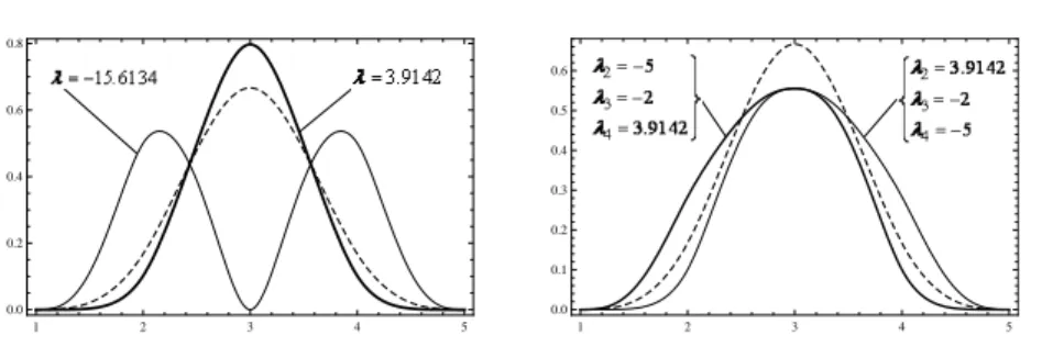
For a uniform knot vector, Figure 2 shows cubic uniform B-spline basis functions (dashed lines) and the CTH B-spline basis functions with all parameters being the same (left)and with all parameters different from one another (right).
1 2 3 4 5 0.0
0.2 0.4 0.6 0.8
1 2 3 4 5
0.0 0.1 0.2 0.3 0.4 0.5 0.6
Figure 2: CTH B-spline basis functions
3. CTH B-spline curves
3.1. Construction of the curves
Definition 3.1. Given control pointsPi ∈Rd(d= 2,3, i= 0,1, . . . , n)and knots u1< u2< . . . < un−1, foru∈[ui, ui+1], i= 0,1, . . . , n, the curves
r(u) =
3
X
j=0
Pi+j−1T Hj,3(t) (3.1)
are defined to be piecewise CTH-B-spline curves, where∆i=ui+1−ui, u= u−∆uii. We can construct the open and closed curves similar to the cubic B-Spline curves.
For open curves, we can expand the curve segment by setting (ee−−1)1)22
−π 6 λ0, λn6 e−1)
2π2
(e−1)2π2−8e,u0< u1, un−1< un, P−1= 2P0−P1, Pn+1= 2Pn−Pn−1.This assures that original points P0 and Pn are the points on the curves, i.e., r(u0) = P0, r(un) = Pn. For closed curves, we can periodically assign control points by setting Pn+1 = P0, Pn+2 = P1, Pn+3 = P2, and expand the knots by setting un−1 < un < un+1 < un+2 and letλi ∈[(ee−−1)1)22
−π,(e−e−1)1)2π22π−28e],i =n, n+ 1, n+ 2, λ1 =λn+2. Thus, the parametric formulae for closed curves are defined on the interval[u1, un+1].
3.2. Properties of the curves
3.2.1. Parametric continuity
Curves (3.1) are piecewise trigonometric hyperbolic polynomial curves. We need to show the continuity of the curves.
Theorem 3.2. For [u1, un−1], curves (3.1) are GC2continuous. The uniform curves (3.1) are C2 continuous.
Proof. Fori= 0,1, . . . , n, We have r(u+i ) = (π−2
2π +λi
π − λi
(e−1)2)(Pi−1+Pi+1) + (2 π−2λi
π + 2λi
(e−1)2)Pi,(3.2)
r(u−i+1) = (π−2 2π +λi+1
π − λi+1
(e−1)2)(Pi+Pi+2) + (2
π−2λi+1
π + 2λi+1
(e−1)2)Pi+1(3.3),
r′(u+i) = 1 2∆i
(Pi+1−Pi−1), (3.4)
r′(u−i+1) = 1 2∆i
(Pi+2−Pi), (3.5)
r′′(u+i ) = (e−1)π+ ((e−1)π−2(e+ 1))λi)
4(e−1)∆2i (Pi−1−2Pi+Pi+1), (3.6)
r′′(u−i+1) =(e−1)π+ ((e−1)π−2(e+ 1))λi+1)
4(e−1)∆2i (Pi−2Pi+1+Pi+2), (3.7) Thus, we obtain
r(k)(u−i ) = ( ∆i
∆i−1
)kr(k)(u+i ), k= 2,3, i= 0,1, . . . , n−2. (3.8)
This implies the theorem.
From (3.4) and (3.5), we know that the tangent line of curves r(u) at the point r(ui)is parallel to the line segment Pi−1Pi+1 (for any λi ). This property corresponds to the property of the cubic uniform B-spline curves.
Theorem 3.3. The curvature of the curves at u=ui is
K(ui) = |(e−1)π+ ((e−1)π−2(e+ 1))λi)|
e−1
|(Pi−Pi−1)×(Pi+1−Pi)|
kPi+1−Pi−1k3 (3.9) Proof. According to (3.4) and (3.6),the curvature of the curves atu=ui is
K(ui) =|r′(ui)×r′′(ui)|
kr′(ui)k3
= |(e−1)π+ ((e−1)π−2(e+ 1))λi)|
e−1
|(Pi+1−Pi−1)×(Pi−1−2Pi+Pi+1| kPi+1−Pi−1k3
= |(e−1)π+ ((e−1)π−2(e+ 1))λi)|
e−1
|(Pi−Pi−1)×(Pi+1−Pi)|
kPi+1−Pi−1k3 .
According to (3.9), the local parameterλi controls the curvature of the curves r(u)at the end of the curve segments. Whenλi> 2(e+1)(e−1)π
−(e−1)π, the curvature of the curves at u=ui increases with the increase of λi. When λi < 2(e+1)(e−−1)π(e−1)π, the curvature of the curves at u=ui increases with the decrease ofλi.
3.2.2. Local and global adjustable properties By rewriting (3.1), foru∈[ui−1, ui], we have
ri−1(u) =T H0,3(t;λi−1)Pi−2+T H1,3(t;λi−1, λi)Pi−1+
T H2,3(t;λi−1, λi)Pi+T H3,3(t;λi)Pi+1. (3.10) Foru∈[ui, ui+1], we have
ri(u) =T H0,3(t;λi)Pi−1+T H1,3(t;λi, λi+1)Pi+
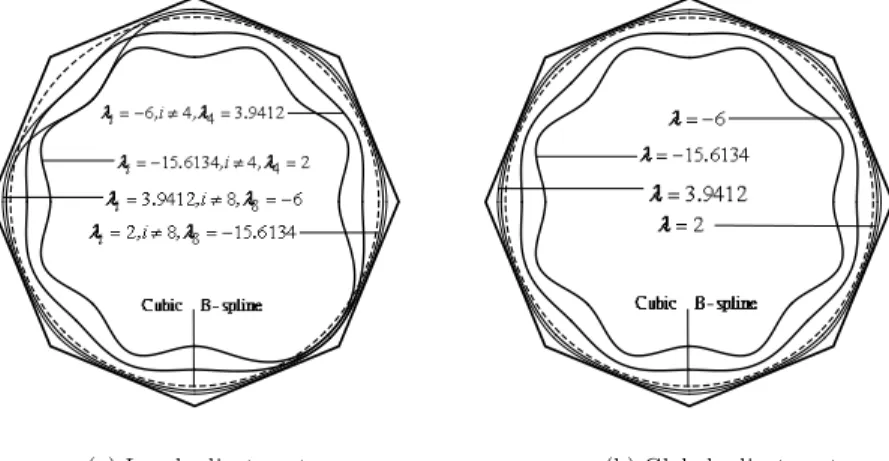
T H2,3(t;λi, λi+1)Pi+1+T H3,3(t;λi+1)Pi+2. (3.11) Obviously, weight parameter λi only affect two curve segments ri−1(u) and ri(u)without altering the remainder, namely, weight parameterλionly affect control polygonPi−\1PiPi+1. So we can adjust the curves locally by changing certain λi. From Figure 3(a), we can see that increasing λi moves locally the curvesr(u)u∈ [ui−1, ui+1]towards the control polygonPi−\1PiPi+1, or decreasingλimoves locally the curvesr(u)u∈[ui−1, ui+1]away the control polygonPi−\1PiPi+1.
(a) Local adjustment (b) Global adjustment
Figure 3: Adjusting the shape of the curves
When all λi are the same, the curves can be adjusted globally. From Figure 3(b), we can see that when the control polygon is fixed, adjusting the value of the weight parameters from -15.6134 to 3.9412, the CTH B-spline curves can cross the
cubic B-spline curves (dashed lines) and reach the both sides of cubic B-splines, in other words, the CTH B-spline curves can range from inside the cubic B-spline curves to outside the cubic B-spline curves. And, the weight parameters are of the property that the larger the weight parameter is, the more closely the curves approximate the control polygon.
3.2.3. Local and global interpolation
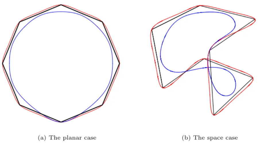
Curve (3.1) can also be used for local interpolation. Letλi= (e2(e−−1)1)22(2−π)
−2π)≈8.91206, from (3.2) and (3.3), we haver(ui) =Pi. This means that curver(u)interpolates point Pi atu=ui locally. Thus, we provide aGC2continuous local interpolation method without solving a linear system or any additional control points. The given piecewise CTH B-spline curves unify the representation of the curves for interpolating and approximating the control polygons.
Obviously, when allλi =2(e(e−−1)1)22(2−π)
−2π), the curve can interpolate the control poly- gon globally. Figure 4 shows global interpolation curves with allλi = (e2(e−−1)1)22(2−π)
−2π)
(red lines) and local interpolation curves with allλi = −1exceptλ5 = (e2(e−−1)1)22(2−π)
−2π)
(blue lines).
(a) The planar case (b) The space case
Figure 4: The local and global interpolation curves
4. The representations of cycloid, helix and catenary
Given uniform knots, when all λi = 0, curves r(u) are piecewise trigonometric polynomial curves. In this case, foru∈[ui, ui+1], if we takePi−1= (π−22a, a), Pi= (0,2−2πa), Pi+1= (2−2πa, a), Pi+2= (2a,2+π2 a) (a6= 0),then the coordinates ofr(u) are
x=a(ti−sinπ2ti), y=a(1−cosπ2ti).
This gives the parametric equation of cycloid. Hence r(u)is an arc of a cycloid, see Figure 5.
Figure 5: The representation of cycloid by the CTH B-spline curves
If we takePi−1= (m, n−π2a,−b), Pi = (m+π2a, n,0), Pi+1= (m, n+π2a, b), Pi+2= (m−π2a, n,2b) (ab6= 0), the coordinates ofr(u)are
x=m+acosπ2ti, y=n+asinπ2ti, z=bti,
which is parametric equation of a helix. Hencer(u)is a helix segment, see Figure 6.
Figure 6: The representation of helix by the CTH B-spline curves
On the other hand, given uniform knots, when all λi = 1, curves r(u) are piecewise hyperbolic polynomial curves. In this case, foru∈[ui, ui+1], if we take Pi−1 = (2a,ee43+1
−ea), Pi= (a,ee22+1
−1a), Pi+1 = (0,e22e
−1a), Pi+2 = (−a,ee22+1
−1a) (a6= 0) , then the coordinates of r(u)are
x=ati, y=acoshti.
This gives the parametric equation of catenary. Hencer(u)is an arc of a catenary, see Figure 7.
Figure 7: The representation of catenary by the CTH B-spline curves
Remark 4.1. By selecting proper control points and weight parameters, some conics such as hyperbola, ellipse and some transcendental curves such as sine curve, cosine curve and hyperbolic sine curves can also be represented via CTH B-spline curves.
5. Application of the curves
As mentioned in section 4, the types of the curves can be changed by selecting control points and parameters properly. So, as an application, we can construct a blending curve using different type curve segments flexibly. For example, given a uniform knot vector, let control points as follows,P0 = (−2,π4), P1 = (π−24,0), P2 = (−2,−π4), P3 = (−π+44 ,0), P4 = (−e22+1,e4+ee33−e+1
−e ), P5 = (−1,e2e2 2
−1), P6 = (0,e2e+2e2 −1
−1 ), P7 = (1,e2e22
−1), P8 = (2,e4+ee33−e+1
−e ), P9 = (1,6), P10 = (2,π+122 ), P11 = (3,6), P12 = (4,122−π), P13 = (4,e2e+1), P14 = (3,1), P15 = (2,0), P16 = (1,−1), P17 = (π−22,1), P18 = (0,2−2π), P19 = (2−2π,1), P20 = (2,2+π2 ). so we obtain a blending curve composed of different type curve segments, which is C2 continuous, see Figure 8.
6. Conclusions
CTH B-spline curves inherited nearly all the properties that CB-spline curves and CH-spline curves and cubic B-spline curves have, such as variation diminishing property, convex hull property, geometric invariance and so on. In this paper, we focus on some special properties of the introduced curves. For example, the shape of the curves can be adjusted globally or locally without adjusting the corresponding control polygon. Without solving system of equations, the curves can interpolate certain control points with proper parameter values. Also, the types of the curves can be switched by weight parametersλi = 0 or1, which are easier to determine than the FB-spline or the UE-spline.
-2 0 2 4 -2
0 2 4 6
Figure 8: AC2continuous blending curve
(a) Adjusting surfaces locally (b) Adjusting surfaces globally
(c) Local interpolation surfaces (d) Global interpolation surfaces
Figure 9: CTH B-spline surfaces
Both rational methods (NURBS or Rational Bézier curves) [15] and CTH B- spline curves can deal with both free form curves and most important analytical shapes for the engineering. However, CTH B-spline curves are simpler in structure and more stable in calculation .The weight parameters of CTH B-spline curves have geometric meaning and are easier to determine than the rational weights in rational methods. Also, CTH B-spline curves can represent the helix, the cycloid, and the catenary precisely, but NURBS can not. Therefore, CTH B-spline curves would be useful for engineering.
Just as in the construction of cubic B-spline tensor product surfaces from cubic B-spline curves, CTH B-spline surfaces can be constructed from CTH B-spline curves easily. And many properties of the curves can be extended to the surfaces.
Figure 9 shows an example of the CTH B-spline tensor product surfaces, where surface shapes are adjusted locally and globally (see (a) and (b)), and surfaces can also interpolate the control mesh locally and globally (see(c) and (d)).
References
[1] Mainar, E., Peña, J.M., Sánchez-Reyes, J., Shape preserving alternatives to the rational Bézier model,Computer Aided Geometric Design, 18 (2001), 37–60.
[2] Zhang, J.W., C-curves: An extension of cubic curves, Computer Aide Geometric Design, 13 (1996), 199–217.
[3] Zhang, J.W., Two different forms of C-B-splines,Computer Aided Geometric Design, 14 (1997), 31–41.
[4] Mainar, E., Peña, J.M., A basis of C-Bézier splines with optimal properties,Com- puter Aided Geometric Design, 19 (2002), 291–295.
[5] Hoffmann, M., Li, Y.J.,Wang, G.Z., Paths of C-Bézier and C-B-spline curves, Computer Aided Geometric Design, 23 (2006), 463–475.
[6] Koch, P.E., Lyche, T., Exponential B-splines in Tension. In: Chui, C.K., Schu- maker, L.L., Ward, J.D. (Eds.), Approximation Theory VI. Academic Press, New York, 1989, 361–364.
[7] Lü, Y.G., Wang, G.Z., Yang, X.N., Uniform hyperbolic polynomial B-spline curves,Computer Aided Geometric Design, 19 (2002), 379–393.
[8] Li, Y.J., Wang, G.Z., Two kinds of B-basis of the algebraic hyperbolic space,Journal of Zhejiang University Science A, 6 (2005), 750–759.
[9] Zhang, J.W., Krause, F.-L., Zhang, H.Y., Unifying C-curves and H-curves by extending the calculation to complex numbers,Computer Aided Geometric Design, 22 (2005), 865-883.
[10] Zhang, J.W., Krause, F.-L., Extend cubic uniform B-splines by unified trigono- metric and hyperbolic basis,Graphic Models, 67 (2005), 100–119.
[11] Hoffmann, M., Juhász, I., Modifying the shape of FB-spline curves, Journal of Applied Mathematics and Computing, 27 (2008), 257–269.
[12] Wang, G.Z. Fang, M.E., Uinfied and extended form of three types of splines, Journal of Computational and Applied Mathematics, 216 (2008), 498–508.
[13] Lin, S.H., Wang, G.Z., Extension of definition interval for C-curves, Journal of Computer Aided Design and Computer Graphics, 17 (2005), 2281–2285 (in Chinese).
[14] Han, X.L., Piecewise quartic polynomial curves with a local weight parameter, Journal of Computational and Applied Mathematics, 195 (2006), 34–45.
[15] Farin, G., Curves and Surfaces for Computer Aided Geometric Design, 4th ed, Academic Press, San Diego, 1997, CA.
Jin Xie
Department of Mathematics and Physics, Hefei University, Hefei 230601, China e-mail: hfuuxiejin@126.com
Jieqing Tan
School of Mathematics, Hefei University of Technology, Hefei 230009, China e-mail: jieqingtan@yahoo.com.cn
Shengfeng Li
Department of Mathematics and Physics, Bengbu College, Bengbu 233000, China e-mail: lsf7679@yahoo.com.cn