Caustics of spline curves ∗
Ede Troll, Miklós Hoffmann
Institute of Mathematics and Computer Science Eszterházy Károly University, Eger, Hungary [troll.ede,hoffmann.miklos]@uni-eszterhazy.hu Submitted September 26, 2017 — Accepted December 18, 2017
Abstract
If we consider a curve as a mirror, then parallel light rays reflected by this mirror curve form a family of lines, which generally has an envelope.
This envelope is called caustic curve of the given mirror curve. The aim of this paper is to describe the caustic curve of a free-form curve and study its alteration by the modification of a control point. We will provide results of general form, and case studies in terms of Bézier and B-spline curves.
Keywords:caustic curve, Bézier curve, B-spline curve
1. Introduction
The classical definition of caustic curves can be found in several books (e.g. in [1, 2]), which can be adapted for parameterical curves as follows.
Definition 1.1. Given a direction vector v(vx, vy) of light rays and the mirror curve r(x(t), y(t)), t∈[0,1], the envelope of rays (if exists) reflected by the curve is called caustic curve (or simply caustic) of the given curve.
More precisely the curve defined above is calledcatacausticcurve, making dis- tinction between reflected and refracted rays – in this latter case the envelope curve is called diacaustic curve. Throughout the paper we will consider only reflected rays, therefore the curve will simply be called caustic.
Although the study of caustic curves has a long history in mathematics and optics, the shape of the mirror is generally a classical curve, such as line, circle
∗This research was supported by the grant EFOP-3.6.1-16-2016-00001 (Complex improvement of research capacities and services at Eszterházy Károly University).
http://ami.uni-eszterhazy.hu
201
or parabola. In the case of reflection by a circle, the caustic is an epicycloid, the locus of a fixed point on the circumference of a circle that rolls on the exterior of another circle, whilst in the case of reflection by the parabola, the caustic is a cubic algebraic curve called Tschirnhausen’s cubic (see e.g. [3]).
But there are limited results in geometric modeling considering caustic curves of other curves, especially caustic curve of free-form curves. While it is relatively easy to visualize the family of rays for any type of mirror curve, and the human perception can ‘realize’ the envelope if the family is dense enough, which can also been approximated numerically providing predefined shapes ([4] and references therein), the exact computation of the caustic curve yielding closed form of these curves is a challenging problem. Exact computation of the evolute of Bézier curves using computer algebra software can be found in [5]. The aim of this paper is to provide exact mathematical description of the caustic curve of free-form mirror curves with arbitrary basis functions in a closed form.
2. The caustic of a free-form curve
In this section we will discuss the method of calculating the caustic of a control point based free-form curve. Let the curve be given in the form
r(t) = Xn
i=0
Ai(t)pi,
wheret∈[0,1],A(t)i are the basis functions and pi are the control points.
When we emit parallel light rays onto the curve with the direction vector v(vx, vy)then these rays will form the family of straight lines
l(u, t) =r(t) +uv,
whereu∈Ris the running parameter of the lines, whiletis the family parameter, coinciding the running parameter of the mirror curve.
To obtain the reflected rays, we have to mirror these incoming rays onto the corresponding tangent lines
t(w, t) =r(t) +wr0(t), wherew∈R.
To define the reflected rays we translated the points of the curve at everytwith the vector v and mirrored them onto the tangent lines. The mirrored points are mr(t) (xm(t), ym(t)), where
xm(t) =x(t)−2hv,nt(t)ixn(t), ym(t) =y(t)−2hv,nt(t)iyn(t),
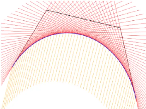
Figure 1: The family of incoming light rays and the corresponding tangents
wherent(t) (xn(t), yn(t))are the unit normal vectors of the tangents and xn(t) = y0(t)
q
x02(t) +y02(t) ,
yn(t) = −x0(t) q
x02(t) +y02(t) .
Now the direction vector of the reflected rays are vr(t) = mr(t)−r(t) and the family of the reflected rays can be described as
lr(u, t) =r(t) +uvr(t), whereu∈Rand the coordinate functions are
xl(u, t) =x(t) +uxvr(t) yl(u, t) =y(t) +uyvr(t).
Figure 2: The family of reflected light rays
To compute the envelope, that is the caustic curve, we have to solve the following
equation foru
∂xl
∂t
∂xl
∂yl ∂u
∂t
∂yl
∂u
= 0, where
∂xl
∂t = 2u
2
vxy02(t)−vyx0(t)y0(t)
(x0(t)x00(t) +y0(t)y00(t)) x02(t) +y02(t)2
− 2vxy0(t)y00(t)−vy(x0(t)y00(t) +y0(t)x00(t)) x02(t) +y02(t)
+x0(t),
∂xl
∂u =vx−2y0(t) (vxy0(t)−vyx0(t)) x02(t) +y02(t) ,
∂yl
∂t = 2u
2
vyx02(t)−vxx0(t)y0(t)
(x0(t)x00(t) +y0(t)y00(t)) x02(t) +y02(t)2
− 2vyx0(t)x00(t)−vx(x0(t)y00(t) +y0(t)x00(t)) x02(t) +y02(t)
+y0(t),
∂yl
∂u =vy−2x0(t) (vyx0(t)−vxy0(t)) x02(t) +y02(t) . Substituting these forms into the original equation
∂xl
∂u
∂yl
∂t −∂yl
∂u
∂xl
∂t = 0
after some calculation the equation can be simplified in the following form 2u vx2(x0(t)y00(t)−y0(t)x00(t)) +v2y(x0(t)y00(t)−y0(t)x00(t))
x02(t) +y02(t) +vy
x03(t) +x0(t)y02(t)
−vx
y03(t) +y0(t)x02(t) x02(t) +y02(t) = 0
and the determinant equation gives us u(t) what is the parameter u of the rays expressed by the family parametert as follows
u(t) =−1 2
vy
x03(t) +x0(t)y02(t)
−vx
y03(t) +x02(t)y0(t) vx2+vy2
(x0(t)y00(t)−x00(t)y0(t)) .
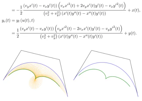
Now we can express the envelope of the reflected rays c(t) (xc(t), yc(t)) as the function of the parametert of the original free-formed curve where
xc(t) =xl(u(t), t)
=−1 2
(vyx0(t)−vxy0(t))
vxx02(t) + 2vyx0(t)y0(t)−vxy02(t) vx2+v2y
(x0(t)y00(t)−x00(t)y0(t)) +x(t), yc(t) =yl(u(t), t)
= 1 2
(vyx0(t)−vxy0(t))
vyx02(t)−2vxx0(t)y0(t)−vyy02(t) v2x+v2y
(x0(t)y00(t)−x00(t)y0(t)) +y(t).
Figure 3: The caustic curve of a control point based free-formed curve
In these computations we extensively used computer algebra softwares. As we can observe from the equation above, the caustic curve of a control point based free formed curve is rational, and its degree depends on the degree of the original basis functions.
Example 2.1. The construction of the caustic curve described in the preceding section is general, that is valid for every control point based free-form curve, and it is independent of the degree and type of the basis functions. Here we provide some case studies of the results for the most popular free-form curves.
In Figure 4 a Bézier curve of degree 4 can be seen in the same position but with different incoming direction of light rays.
Since the caustic has the same parameter intervalt∈[0,1]as the original curve, the piecewisely computed caustics of connect B-Spline arcs will also be smoothly connected automatically. In Figure 5 a uniform cubic B-Spline and its piecewisely connected caustic curve can be seen. To show the arcs of the caustics we drew them with different colours.
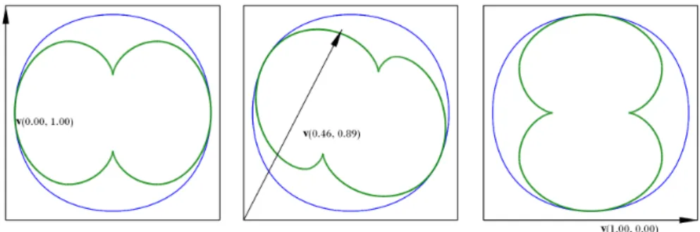
The last example shows a closed uniform cubic B-Spline and its caustics with various light ray directions, where the control points are vertices of a square (Fig 6).
In the leftmost image the incoming rays are parallel to they axis, while in the right image the rays are parallel to the xaxis. These caustics look very similar to the nephroid what is the caustic of the circle. In the middle image the direction vector of the incoming rays does not parallel to any of the axes and because the cubic B-Spline can not describe an exact circle, the caustic is slightly distorted.
Figure 4: The caustic of a Bézier curve of degree 4 with different light directions
Figure 5: The caustic curve of the uniform cubic B-spline curve (different colours means different arcs of the caustic)
Figure 6: The caustic of the closed uniform cubic B-Spline curve with different light ray directions
2.1. Geometric effect of the control points
In this section, our aim is to describe the alteration of the caustic curve by the modification of a control point. This means that we would like to compute the path
of a pointc(t0), t0∈[0,1]of the caustic curve when a control pointpi, i∈0,1, . . . , n moves along a straight line. To describe the effect of the modification we have to express the caustic curve in a way that the running parameter t is considered to be constant (t = t0), and the control point pi(xpi, ypi) is the parameter (more precisely, the coordinates of the control point are the parameters) of the path. To emphasize this fact the path of the point c(t0) is denoted by s(t0,pi). Let us express the coordinate functions of the free-form curve and their derivatives as a constant part plus the part depending on the coordinates of the moving control points:
x(t0, xpi) =X
j6=i
Aj(t0)xpj +Ai(t0)xpi, y(t0, ypi) =X
j6=i
Aj(t0)ypj+Ai(t0)ypi, x0(t0, xpi) =X
j6=i
A0j(t0)xpj +A0i(t0)xpi, y0(t0, ypi) =X
j6=i
A0j(t0)ypj+A0i(t0)ypi, x00(t0, xpi) =X
j6=i
A00j(t0)xpj +A00i(t0)xpi, y00(t0, ypi) =X
j6=i
A00j(t0)ypj +A00i(t0)ypi, wherej runs from 0 to n.
Using the expressions above we can expand the coordinate functions of the caustics in the form
xc(t0, xpi) =−1 2
(vyx0(t0, xpi)−vxy0(t0, xpi)) vx2+v2y
(x0(t0, xpi)y00(t0, xpi)−x00(t0, xpi)y0(t0, xpi))
×
vxx02(t0, xpi) + 2vyx0(t0, xpi)y0(t0, xpi)−vxy02(t0, xpi) vx2+vy2
(x0(t0, xpi)y00(t0, xpi)−x00(t0, xpi)y0(t0, xpi)) +x(t0, xpi),
yc(t0, ypi) = 1 2
(vyx0(t0, ypi)−vxy0(t0, ypi)) v2x+v2y
(x0(t0, ypi)y00(t0, ypi)−x00(t0, ypi)y0(t0, ypi))
×
vyx02(t0, ypi)−2vxx0(t0, ypi)y0(t0, ypi)−vyy02(t0, ypi) vx2+vy2
(x0(t0, ypi)y00(t0, ypi)−x00(t0, ypi)y0(t0, ypi)) +y(t0, ypi).
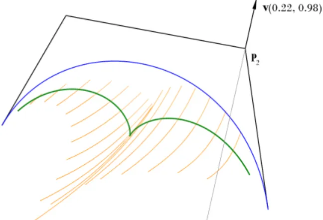
By these expressions we can observe that the pathss(t0,pi)are rational curves (see Fig. 7) and their coordinate functionssx andsy can be expressed as
sx(t0, xpi) = a1x3pi+a2x2pi+a3
a4xpi+a5 , sy(t0, ypi) = b1yp3i+b2yp2i+b3
b4ypi+b5
,
whereak andbk,(k∈ {1,2, . . . ,5})are constants depending on the direction vector of the incoming rays, the fixed value of the running parametert0 and the position of the other control points.
Figure 7: The geometric effect of the alteration of the control point p2 on the caustic curve and paths of points of a cubic Bézier curve when the control point moves along the straight line defined by the
direction vectord(0.22,0.98)
3. Conclusion and future research
Caustic curves of control point based free-form curves have been computed and provided in closed form in this paper. The theoretical results hold for any free- form curve, independently of its specific basis functions. Beside these results, some examples of the most popular free-form curves are also considered. As an important aspect of the design of free-form mirrors and their caustics we have seen, that the alteration of a control point will evidently affect the shape of the caustic, and fixed points of the caustic curve move along rational curves as one of the control points is altered along a straight line.
These results may form the basis for the spatial extension of the computation of caustics of free-form surfaces, which is an important aspect of geometric modeling and free-form architecture as well. It can be the direction of our future research.
References
[1] Lawrence, J. D., A Catalog of Special Plane Curves, New York: Dover, 1972.
[2] Lockwood, E. H., A Book of Curves, Cambridge University Press, 1967, pp. 182–
185.
[3] Farouki, R. T., Pythagorean-Hodograph Curves: Algebra and Geometry Insepara- ble, Springer, 2008.
[4] Schwartzburg, Y., Testuz, R., Tagliasacchi, A., Pauly, M., High-contrast computational caustic design, ACM Transactions on Graphics (TOG), 33(4) (2014), 1–11.
[5] Tsukada, T., Caustics on Spline Curves, Wolfram Demonstration Project http:
//demonstrations.wolfram.com/CausticsOnSplineCurves/ (visited on: December 13, 2017).
[6] Fowler, B., Bartels, R., Constraint-based curve manipulation, IEEE Comp.
Graph. and Appl., Vol. 13 (1993), 43–49.