A limit theorem for one-parameter alteration of two knots of B-spline curves

32(2005) pp. 53–60.

A limit theorem for one-parameter alteration of two knots of B-spline curves ^∗

Miklós Hoffmann

, Imre Juhász

aInstitute of Mathematics and Computer Science Károly Eszterházy College

e-mail: hofi@ektf.hu

bDepartment of Descriptive Geometry University of Miskolc e-mail: agtji@gold.uni-miskolc.hu

Abstract

Knot modification of B-spline curves is extensively studied in the past few years. Altering one knot value, curve points move on well-defined paths, the limit of which can be computed if the knot value tends to infinity. Symmetric alteration of two knot values can also be studied in a similar way. The extension of these limit theorems for general synchronized modification of two knots is discussed in this paper.

Key Words: B-spline curve, knots, paths AMS Classification Number: 68U05

1. Introduction

B-spline curves and surfaces are well-known geometric modeling tools in com- puter aided design. The definition of the k^th order B-spline curve is as follows (c.f.[13]):

Definition 1.1. The curves(u)defined by s(u) =

Xn

l=0

dlN_l^k(u), u∈[uk−1, un+1]

∗This research was supported by the Hungarian National Research Fund (OTKA) grant No.

T 048523.

53

is called B-spline curve of orderk6n(degreek−1), where the pointsdlare called control points or de Boor-points, whileN_l^k(u)is thek^thnormalized B-spline basis function, given by the following recursive functions:

N_j¹(u) =

½ 1 if u∈[uj, uj+1), 0 otherwise N_j^k(u) =_u ^u−uj

j+k−1−ujN_j^k−1(u) +_u^uj+k−u

j+k−uj+1N_j+1^k−1(u).

The numbersuj6uj+1∈Rare called knot values or simply knots, and0/0 ˙=0by definition.

In the last few years several papers dealt with knot modification of B-spline curves.

From a practical point of view, optimization techniques by changing the entire knot vector have been studied in [1] and [3], while shape control algorithms for cubic B-spline curves by changing three consecutive knots have been described in [10].

Basic theoretical results of alteration of a single knot value can be found in [8]

and [9], where the notion of path has been introduced for curvess(u, ui)obtained by fixing the parameter value u and modifying the knot ui. In [8] the authors proved that these paths are rational curves. In [5] these paths are extended in a way that monotonicity of knot values was not fulfilled, i.e. we let ui < ui−1

and ui > ui+1. Here we emphasize that this extension is a pure mathematical construction that is, the functions N_l^k(u) obtained by this substitution are not basis functions any more. This extension, however can help us to examine the limit properties of paths. These extended paths have been studied in [5] where the following theorem has been proved:

Theorem 1.2. Modifying the single multiplicity knotu_iof the B-spline curves(u), points of the extended paths of s(u), u∈[ui−1, ui+1)tend to the control points di

anddi−k asui tends to−∞and∞, respectively, i.e.,

uilim→−∞s(u, ui) =di, lim

ui→∞s(u, ui) =di−k,∀u∈[ui−1, ui+1).

Some of the results of knot modification have been successfully extended for B- spline surfaces as well (c.f. [4], [11]).

2. Alteration of two knots

Similarly to the previous section, one can modify two (not necessarily neigh- boring) knots ofs(u)as well. Let us denote the two altered knots byui andui+z, ((k−1)< i < i+z <(n+ 1)). If their modification is independent of each other, the possible positions of each fixed point of the curve can be described as a planar region. However if the modification of the two knots is synchronized in a way that their movement depend on a single parameter, the points of the curve will move on paths. In [6] the modification of typeui+λand ui+z−λ has been discussed and the following result has been proved.

Theorem 2.1. Symmetrically altering the knots ui and ui+z (z ∈ {1,2, . . . , k}, wherekis the order of the original B-spline curve), extended paths of points of the arcssj,(j=i, i+ 1, . . . , i+z−1)converge to the midpoint of the segment bounded by the control pointsdi anddi+z−k when λ→ −∞, i.e.

λ→−∞lim s(u, λ) = di+di+z−k

2 , u∈[ui, ui+z). (2.1) In this paper we extend this result for a more general movement of knots. Let the modification of the two knots be described by the following way:

ui = ui+tλ uj = uj−(1−t)λ,

wheret∈[0,1]is fixed andλ∈Ris a running parameter. If one intend to preserve the monotonicity of the knot values, onlyλ ∈[−c, c], c = min{ui−ui−1, ui+1− ui, uj−uj−1, uj+1−uj} is allowed, but in case of extended paths the parameter can be any real number.

3. The limit theorem

For the synchronized motion described in the previous section the following statement holds.

Theorem 3.1. Modifying the knots

ui=ui+tλ, ui+z=ui+z−(1−t)λ, (z= 1,2, . . . , k) (3.1) the points of the extended paths of s(u), u∈[ui, ui+z) tend to a point of the line segmentdidi+z−k the barycentric coordinates of which are tand(1−t), i.e.

λ→−∞lim s(u, t, λ) =tdi+ (1−t)di+z−k, u∈[ui, ui+z), t∈[0,1].

Proof. At first we prove that ifu∈[ui, ui+z), then forz= 1,2, ..., k−1

λ→−∞lim N_i+z−k^k (u, t, λ) = (1−t)

λ→−∞lim N_i^k(u, t, λ) = t

λ→−∞lim N_j^k(u, t, λ) = 0, (j6=i, i+z−k), and forz=k

λ→−∞lim N_i^k(u, t, λ) = 1

λ→−∞lim N_j^k(u, t, λ) = 0, (j6=i).

We prove the statement by induction on k. For the sake of simplicity the variables of the basis functions are omitted.

i) k= 3

On the interval[ui, ui+1)the basis function is of the following form N_i³= u−ui

ui+2−ui

u−ui

ui+1−ui.

d4

d6

15 0.

t=

d4

d6

5 0.

t=

d4

d6

85 0.

t=

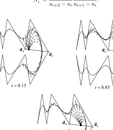
Figure 1: A cubic (k = 4) B-spline curve and its paths for various values of t, (i= 6, z= 2).

Substituting equations (3.1) into this function the numerator as well as the denominator will be quadratic in λ. The main coefficient of the numerator ist² independently of z. For z = 1 the main coefficient in the denominator can be calculated by applying

ui+2−ui = ui+2−(ui+tλ) =ui+2−ui−tλ

ui+1−ui = ui+1−(1−t)λ−(ui+tλ) =ui+1−ui−λ which turn to bet, while forz= 2applying

ui+2−ui = ui+2−(1−t)λ−(ui+tλ) =ui+2−ui−λ

ui+1−ui = ui+1−(ui+tλ) =ui+1−ui−tλ

the main coefficient istagain. Ifz= 3, then due toui=ui+tλthe main coefficient ist². Thus we obtain, that

λ→−∞lim N_i³=

½ t, ifz= 1,2

1, ifz= 3 u∈[ui, ui+1). On the interval[ui, ui+1)the other two basis functions are of the form

N_i−2³ = ui+1−u ui+1−ui−1

ui+1−u ui+1−ui

N_i−1³ = u−ui−1

ui+1−ui−1

ui+1−u

ui+1−ui + ui+2−u ui+2−ui

u−ui

ui+1−ui.

Similar calculation leads to the main coefficients and to the limits of these two functions, which are (1−t) and 0 for z = 1, 0 and (1−t) for z = 2 while 0 in both cases forz= 3. For the rest of the indices (j 6=i−2, i−1, i)N_j³≡0 always holds. Thus the proof is ready fork= 3on the interval[ui, ui+1). For the intervals [ui+1, ui+2)and[ui+2, ui+3)the statement can be proved in an analogous way.

ii) Suppose that for∀u∈[ui, ui+z)

λ→−∞lim N_i^k−1 =

½ t, ifz= 1, ..., k−2

1, ifz=k−1 (3.2a)

λ→−∞lim N_i+z−k+1^k−1 =

½ (1−t), ifz= 1, ..., k−2

1, ifz=k−1 (3.2b)

λ→−∞lim N_j^k−1 = 0,(j 6=i, i+z−k+ 1), ifz= 1, ..., k−1. (3.2c) holds. At first we prove that the assumptions (3.2a)-(3.2c) yield

λ→−∞lim N_i^k=

½ t, ifz= 1, ..., k−1

1, ifz=k u∈[ui, ui+z). (3.3) By definition

N_i^k(u) = u−ui

ui+k−1−ui

N_i^k−1(u) + ui+k−u ui+k−ui+1

N_i+1^k−1(u).

Due to (3.2a) the limit of the first term istifz≤k−2. Ifz= 1thenN_i+1^k−1(u)≡0, thus the limit of the second term equals0,while forz = 2, ..., k−2 the limit also equals 0 due to (3.2c). For z = k−1 the limit of the fraction in the first term equalst since

u−ui = u−ui−tλ

ui+k−1−ui = ui+k−1−λ+tλ−ui−tλ=ui+k−1−ui−λ.

But (3.2a) yields lim

λ→−∞N_i^k−1= 1, thus the limit of the first term istagain. Taking into account equation (3.2c) the limit of the second term is0.

Finally, forz=kthe proof is analogous to that of Theorem 1.2, thus we proved (3.3).

Now applying (3.2a)-(3.2c) we verify

λ→−∞lim N_i+z−k^k =

½ (1−t), ifz= 1, ..., k−1

1, ifz=k u∈[ui, ui+z). (3.4) By definition

N_i+z−k^k (u) = u−ui+z−k

ui+z−1−ui+z−k

N_i+z−k^k−1 (u) + ui+z−u ui+z−ui+z−k+1

N_i+z−k+1^k−1 (u). Due to (3.2c) the limit of the first term equals 0 for z ≤ k −1. The limit of the fraction in the second term is 1 for z = 1, ..., k−2, while (3.2b) yields

λ→−∞lim N_i+z−k+1^k−1 (u) = (1−t). Forz=k−1applying ui+k−1−u = ui+z−(1−t)λ−u

ui+k−1−ui = ui+k−1−λ+tλ−ui−tλ=ui+k−1−ui−λ

the limit of the fraction in the second term equals (1−t), while due to (3.2b)

λ→−∞lim N_i+z−k+1^k−1 (u) = 1. Thus the limit of the second term is always equal to (1−t). The casez=k is analogous to the proof of Theorem 1.2 again, thus (3.4) is verified.

d6

d5

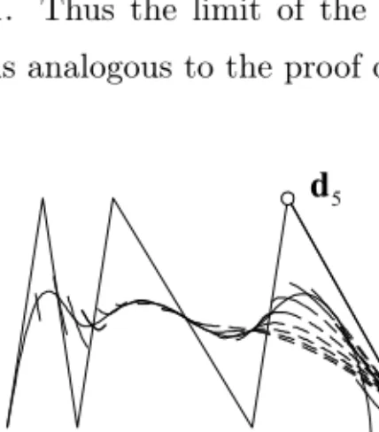
Figure 2: A quadric (k= 5) B-spline curve and its paths fort= 0.85, (i= 6, z= 4).

Finally, we prove that assuming (3.2a)-(3.2c)

λ→−∞lim N_j^k = 0,(j6=i, i+z−k),∀z, u∈[ui, ui+z) (3.5)

holds. By definition

N_j^k(u) = u−uj

uj+k−1−ujN_j^k−1(u) + uj+k−u

uj+k−uj+1N_j+1^k−1(u).

The limit of the first term equals0 (if j =i+z−k+ 1 then j+k−1 =i+z, thus the limit of the fraction is 0, while for the other cases the limit of the basis function in the first term is0 due to (3.2c)). The limit of the second term equals 0as well, (forj+ 1 =ithe limit of the fraction equals 0, while for the rest of the cases (3.2c) yields lim

λ→−∞N_j+1^k−1(u) = 0). Thus (3.5) has also been verified and this

completes the proof. ¤

Figure 1 demonstrates the result for cubic curves, while Figure 2 shows an example for a higher order curve.

References

[1] Aszódi, B., Czuczor, Sz., Szirmay-Kalos, L., NURBS fairing by knot vector optimization,Journal of WSCG, Vol. 12 (2004), 19–26.

[2] Boehm, W., Inserting new knots into B–spline curves, Computer–Aided Design, Vol. 12 (1980), 199–201.

[3] Goldenthal, R., Bercovier, M., Spline curve approximation and design by op- timal control over the knots, Computing, Vol. 72 (2004), 53–64.

[4] Hoffmann, M., Juhász, I., Geometric aspects of knot modification of B-spline surfaces,Journal for Geometry and Graphics, Vol. 6 (2002), 141–149.

[5] Hoffmann, M., Juhász, I., On the knot modification of a B-spline curve, Publi- cationes Mathematicae Debrecen, Vol. 65 (2004), 193–203.

[6] Hoffmann, M., Juhász, I.,Symmetric alteration of two knots of B-spline curves, Journal for Geometry and Graphics, Vol. 9 (2005), 43–49.

[7] Juhász, I.,A shape modification of B-spline curves by symmetric translation of two knots,Acta Acad. Paed. Agriensis, Sect. Math., Vol. 28 (2001), 69–77.

[8] Juhász, I., Hoffmann, M., The effect of knot modifications on the shape of B- spline curves,Journal for Geometry and Graphics, Vol. 5 (2001), 111–119.

[9] Juhász, I., Hoffmann, M., Modifying a knot of B-spline curves,Computer Aided Geometric Design, Vol. 20 (2003), 243–245.

[10] Juhász, I., Hoffmann, M., Constrained shape modification of cubic B-spline curves by means of knots,Computer-Aided Design, Vol. 36 (2004), 437–445.

[11] Li Yajuan, Wang Guozhao, On Knot Modification of B-Spline and NURBS Sur- face,Journal of Computer-Aided Design & Computer Graphics, Vol. 17 (2005), 986–

989.

[12] Piegl, L., Modifying the shape of rational B-splines. Part 1: curves, Computer–

Aided Design, Vol. 21 (1989), 509–518.

[13] Piegl, L., Tiller, W.,The NURBS book, Springer–Verlag, (1995).

Miklós Hoffmann

Institute of Mathematics and Computer Science Károly Eszterházy College

Leányka str. 4.

H-3300 Eger Hungary Imre Juhász

Department of Descriptive Geometry University of Miskolc

H-3515 Miskolc-Egyetemváros Hungary