VIKT ´ORIA F ¨OLDV ´ARI
Abstract. According to the idea of Ozsv´ath, Stipsicz and Szab´o, we define the knot invariant Υ without the holomorphic theory, using constructions from grid homology. We develop a homology theory using grid diagrams, and show that Υ, as introduced this way, is a well-defined knot invariant. We reprove some important propositions using the new techniques, and show that Υ provides a lower bound on the unknotting number.
1. Introduction
In 2014, Ozsv´ath, Stipsicz and Szab´o [11] introduced the knot invariant Υ using knot Floer homology.
In their book [10] they used grid homologies to develop the concordance invariant τ first defined in [9], and among other open problems they presumed that Υ can also be defined without the holomorphic theory.
This idea is reasonable and important: for example the fact thatυ(K) = ΥK(1) gives a lower bound on the unoriented four-ball genus [12], have only been proved using methods based on grid diagrams. Our aim is to work out this new approach: to develop a homology theory using grid diagrams of knots, and to introduce the knot invariant Υ using grid homologies. The significance of this new definition is that it gives the opportunity to examine problems combinatorically. We reprove some important properties using the new techniques.
Former versions of grid diagrams have been studied for more than a century as convenient tools for understanding knots and links [2, 3, 4, 5, 7]. Since every oriented link can be represented by a grid diagram (see [10, Chapter 3.] for the basic definitions), this theory has the advantage of handling knots and links with discrete methods. In the second half of the twentieth century, knot theory was connected with more and more different areas of mathematics, which led to outstanding results.
In recent years, knot theory has undergone significant progress, mostly because of the incorporation of algebraic concepts, such as knot Floer homology, Heegaard Floer homology, Khovanov homology and the generalizations of knot polynomials. Grid diagrams have also been reconsidered [6, 8, 13] to build up grid homology theories which enabled us to approach problems algebraically.
The main points of this paper are the new introduction of Υ in Definition 5.1, and Theorem 5.2 stating that Υ, as defined using grids, is a well-defined knot invariant. In Corollary 5.10 we give a lower bound on the unknotting number. Note that the results were known earlier [11] but their proof was based on the holomorphic theory.
Before proceeding further, we state here some properties of ΥK : [0,2]→Rthat are proved in [11].
• ΥK is additive under connected sum of knots:
ΥK1#K2(t) = ΥK1(t) + ΥK2(t).
• For the mirror image m(K) of the knotK, Υm(K)(t) =−ΥK(t).
• ΥK(t) = ΥK(2−t).
• Suppose thatK1andK2are two knots that can be connected by a genusgcobordism in [0,1]×S3. Then fort∈[0,1]
|ΥK1(t)−ΥK2(t)| ≤t·g.
• For a knotK andt∈[0,1] the invariant ΥK(t) bounds the slice genusgs(K) ofK:
|ΥK(t)| ≤t·gs(K).
1
arXiv:1903.05893v1 [math.GT] 14 Mar 2019
• For an alternating knot K, the ΥK invariant can be explicitly computed:
ΥK(t) = (1− |t−1|)·σ 2, whereσ is the signature of the knotK.
• ΥK(0) = 0 and ΥK(2) = 0.
• Form, n∈N>0, the quantity ΥK(mn) lies in 1nZ.
• The function ΥK :t7→ΥK(t) is continuous and piecewise linear. Each slope is an integer.
• The slope of ΥK(t) att= 0 is given by−τ(K), whereτ is a knot invariant, defined in Chapter 6 of [10].
• If the knots K1 andK2 can be connected with a concordance, then ΥK1(t) = ΥK2(t) for t ∈[0,2].
Furthermore, [K]7→ ΥK is a group homomorphism from the concordance group to the space C = C0[0,2] of continuous functions on [0,2].
For torus knots, the Alexander polynomial [1] determines ΥK(t), see [11].
Acknowledgement: I am grateful to my supervisor, Andr´as Stipsicz, for his help and corrections.
2. Background
2.1. Planar and toric grid diagrams. A planar grid diagram Gwith grid number n is a square on the plane withn rows and ncolumns of small squares (i.e. an n×ngrid), marked with X’s andO’s in a way that no square contains bothX andO, and each row and each column contains exactly oneX and one O.
We use the notation X for the set of squares marked with an X, and Ofor the ones containing an O.
Sometimes we label the markings: {Oi}ni=1,{Xi}ni=1.
We usually work with atoroidal grid diagram, which can be obtained by identifying the opposite sides of a planar grid diagram: its top boundary segment with its bottom one and its left boundary segment with its right one. A planar realization of a toroidal grid diagram is a planar grid diagram obtained by cutting up the toroidal grid diagram along a horizontal and a vertical line.
Every grid diagramGdetermines a diagram of an oriented link in the following way: In each row connect the O-marking to the X-marking, and in each column connect the X-marking to the O-marking with an oriented line segment, such that the vertical segments always pass over the horizontal ones. This way we get closed curves: the diagram of the oriented linkL~ given by the grid diagram. We callGagrid diagram for L.~ The converse is also true: Every oriented link inS3can be represented by a grid diagram. (See [10, Chapter 3.] for the easy proof.)
Acyclic permutationof a planar grid diagramGis a process in which we permute the rows or the columns ofGcyclically. Note that a cyclic permutation has no effect on the induced toroidal grid diagram, and that two different planar realizations of a toroidal grid diagram can always be connected by a sequence of cyclic permutations. Also ~L, represented by the grid diagram stays the same after some cyclic permutations.
2.2. Grid moves. In 1995 Cromwell [3] introduced a list of alterations of grid diagrams that are similar to Reidemeister moves for knot diagrams, and do not change the knot type.
First we consider the two main types of moves on planar grid diagrams, then we extend these to toroidal grid diagrams. For a detailed introduction of grid moves see [10, Chapter 3.].
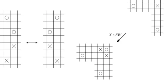
In a grid diagramGevery column determines a closed interval of real numbers that connects the height of its O-marking with the height of its X-marking. Consider a pair of consecutive columns inG, and suppose that the two intervals associated to them are either disjoint, or one is contained in the other (Figure 1). We say that the diagramG0differs fromGby acolumn commutation, if it can be obtained by interchanging two consecutive columns ofGthat satisfy the above condition. Arow commutationis defined analogously, using rows in place of columns. Column or row commutations collectively are calledcommutation moves.
If we consider two consecutive columns in the grid diagramG, such that the interior of their corresponding intervals are not disjoint, but neither is contained by the other, and interchange these columns to get grid diagram G0, then Gand G0 are related by across-commutation. We use the same name for the procedure
interpreted on rows in place of columns. IfL~ andL~0 are two links whose grid diagrams GandG0 differ by a cross-commutation, thenL~ andL~0 are related by acrossing change.
While commutation moves preserve the grid number, the second type of grid moves will change it:
LetGbe ann×ngrid diagram. We say that the (n+ 1)×(n+ 1) grid diagramG0 is thestabilization of Gif it can be obtained fromGin the following way: Choose a marked square inG, and erase the marking in it, in the other marked square in its row and in the other marked square in its column. Then split the row and the column of the chosen marking inGinto two, that is, add a new horizontal and a new vertical line to get an (n+ 1)×(n+ 1) grid, see Figure 1. Note that there are four ways to insert markings in the two new rows and columns to have a grid diagram,G0 can be any of these four.
The following lemma can be found as Lemma 3.2.2. in [10].
Lemma 2.1. Any stabilization can be expressed as a stabilization of the type shown in Figure 1 followed by a sequence of commutations.
Figure 1. A commutation (left) and a stabilization (right)
The inverse of a stabilization is adestabilization. Commutation, stabilization and destabilization together are called grid moves or Cromwell moves.
The following theorem of Cromwell [3] shows us that grid moves and grid diagrams are really effective tools for creating knot invariants:
Theorem 2.2. Two toroidal grid diagrams represent equivalent links if and only if there is a finite sequence of grid moves that transform one into the other.
Grid moves can be transmitted naturally for the case of toroidal grid diagrams: two toroidal grid diagrams differ by a commutation move/a stabilization, if they have planar realizations that differ by a commutation move/a stabilization.
2.3. Grid states and gradings. We would like to define a version of grid homology, so first we need a chain complex. We recall here the concept of grid states, then, for the boundary map, we take rectangles connecting grid states. For a detailed introduction see [10, Chapter 4.].
A grid statex for a grid diagramGwith grid numbern consists ofnpoints in the torus such that each horizontal and each vertical circle contains exactly one element ofx. The set of grid states forGis denoted byS(G).
Consider two grid states x,y∈ S(G) that overlap inn−2 points in the torus. The four points left out are the corners of an embeddedrectangle r, that inherits an orientation from the torus. The boundary of r
is the union of oriented arcs, two of which are on the horizontal and two on the vertical circles. We say that the rectangle r goes from x to y if the horizontal segments in ∂r point from the components of x to the components of y, while the vertical segments point from the components ofyto the components ofx.
Forx,y∈S(G), we use the notation Rect(x,y) for the set of rectangles going fromxtoy.
We call a rectangler∈Rect(x,y) anempty rectangleif
x∩Int(r) =y∩Int(r) =∅.
The set of empty rectangles fromxto yis denoted by Rect◦(x,y).
We will need a generalization of the rectangle idea: Forx,y∈S(G) a (positive)domain ψfromxto yis a formal linear combination of the small squares ofG, where the coefficients are non-negative integers, and the horizontal boundary segments of ψpoint from the components of xto the components of y. The set of domains from xtoyis denoted byπ(x,y).
To introduce grid homology, we equip grid states with two gradings, called the Maslov (MO) and the Alexander grading (A). For the definitions and properties see [10, Section 4.3.]. Here we only state two important facts:
Proposition 2.3. Let Gbe a toroidal grid diagram for a knot, and x,y∈S(G)two grid states that can be connected by some rectangle r∈Rect(x,y). Then,
(1) MO(x)−MO(y) = 1−2· |r∩O|+ 2· |x∩Int(r)|, and (2) A(x)−A(y) =|r∩X| − |r∩O|.
3. The t-modified grid complex
First of all, we recall some basic notions that will play an important role afterwards.
A setS⊂Ris called well-ordered, if every subset ofS has a minimal element. We will use the notation R0={X
α∈A
Uα|A⊂R≥0, Ais well−ordered}
for thelong power series ring over F2. (We denote byF2 the field with two elements.)
R0 is indeed a ring with the following operations: ForA,B ⊂R≥0 well-ordered sets leta= P
α∈A
Uα and b= P
β∈B
Uβ. Define the sum onR0 in a way thata+b= P
γ∈C
Uγ, whereC=A∪B\A∩B is the symmetric difference of the index sets.
Notice that C is well-ordered, since the union, the intersection and the difference of well-ordered sets are also well-ordered.
The multiplication on R0 is defined as the Cauchy-product of the elements, that is,
X
α∈A
Uα
!
·
X
β∈B
Uβ
= X
γ∈A+B
X
α∈A,β∈B α+β=γ
Uγ
.
Here A+B is the sumset of A andB. This definition makes sense, because every γ can be written as the sum of someαandβ in finitely many ways: if we suppose the opposite, then there exists an infinite, strictly decreasing sequence of either the α’s or theβ’s, which contradicts the fact that A and B are well-ordered sets.
LetRt≤ R0 be the subring generated by the elementsUtandU2−t.
Now we are ready to define the chain complex which will give us the desired homologies.
Definition 3.1. For eacht∈[0,2]we define the t-modified grid complextGC−(G)as the free module over Rgenerated by S(G), equipped with theR-module endomorphism∂t−, whose value on anyx∈S(G)is given
by
(3) ∂t−(x) = X
y∈S(G)
X
r∈Rect◦(x,y)
Ut·|X∩r|+(2−t)·|O∩r|
·y.
Theorem 3.2. The operator∂t−: tGC−(G)→tGC−(G) satisfies∂t−◦∂−t = 0.
Proof. We follow the proof of Lemma 4.6.7 in [10]. Consider grid states x and z. For a fixed ψ ∈ π(x,z) denote byN(ψ) the number of ways we can decomposeψas a juxtaposition of two empty rectanglesr1∗r2. Notice that ifψ=r1∗r2for some r1∈Rect◦(x,y) andr2∈Rect◦(y,z), then
|X∩ψ|=|X∩r1|+|X∩r2| and |O∩ψ|=|O∩r1|+|O∩r2|.
It follows that the endomorphism∂t−◦∂t− can be expressed onxas
∂t−◦∂−t (x) = X
z∈S(G)
X
ψ∈π(x,z)
N(ψ)·Ut·|X∩ψ|+(2−t)·|O∩ψ|
·z.
Take a pair of empty rectangles r1 ∈ Rect◦(x,y) and r2 ∈ Rect◦(y,z) so that N(ψ) >0 holds for the domainr1∗r2=ψ. There are three basic cases (see Figure 4.4 in [10] for an illustration):
• x\(x∩z) consists of 4 elements. Then,r1andr2 do not share any common corners. In this case,ψ can only be decomposed as r1∗r2 orr2∗r1. Therefore,N(ψ) = 2.
• x\(x∩z) consists of 3 elements. In this case, the local multiplicities of ψ are all 0 or 1. The corresponding region in the torus is a hexagon with five corners of 90◦, and one of 270◦. NowN(ψ) = 2 again, and the two decompositions can be obtained by cuttingψat the 270◦corner horizontally and vertically.
• x =z. In this case,r1 andr2 intersect along two edges, andψ is an annulus. Since the rectangles are empty, the height or width of this annulus is 1 (called a thin annulus), and N(ψ) = 1. Hence
|X∩ψ|=|O∩ψ|= 1.
Contributions from the first two cases cancel in pairs, because we are working modulo 2. So it is enough to consider the terms whereψis a thin annulus. Note that every thin annulus is a proper choice forψ. Now we have
∂t−◦∂t−(x) =
X
ψis a thin annulus
N(ψ)·U2
·x= 2n·U2·x= 0.
Let us introduce a grading on the preferred basis oftGC−G.
Definition 3.3. Forx∈S(G)the t-gradingof Uα·x is defined as grt(Uα·x) =M(x)−t·A(x)−α, whereM is the Maslov and Ais the Alexander function on grid states.
Proposition 3.4. The differential∂t− drops thet-grading by one.
Proof. Let x ∈ S(G), and consider a non-zero termUt·|X∩r|+(2−t)·|O∩r|·y of the sum in the definition of
∂t−(x) in (3). Sincer∈Rect◦(x,y), from (1) and (2) we know that M(y) =M(x)−1 + 2· |O∩r| and
A(y) =A(x)− |X∩r|+|O∩r|.
Therefore,
grt(Ut·|X∩r|+(2−t)·|O∩r|·y) =M(y)−t·A(y)−t· |X∩r| −(2−t)· |O∩r|=
= (M(x)−1 + 2· |O∩r|)−t·(A(x)− |X∩r|+|O∩r|)−t· |X∩r| −(2−t)· |O∩r|=
=M(x)−t·A(x)−1 = grt(x)−1.
LettGCd−(G) denote the vector space overF2 generated by those monomialsUα·x, wherex∈S(G) and grt(Uα·x) =d. Ifx∈tGC−(G) lies intGCd−(G) for somed, we say thatxishomogeneous.
We can define the homology of (tGC−(G), ∂−t):
Definition 3.5.
tGHd−(G) = Ker(∂−t )∩tGCd−(G)
Im(∂t−)∩tGCd−(G) tGH−(G) =M
d
tGHd−(G).
4. Invariance
4.1. Commutation invariance. The aim of this section is to prove thattGH− is invariant under commu- tation. We introduce the same notations as Section 5.1 in [10].
Theorem 4.1. LetGandG0 be two grid diagrams that differ by a commutation move. Then tGH−(G)∼=tGH−(G0)
as gradedRt-modules.
Proof. Consider two toroidal grid diagramsGandG0with grid numbern, such that this latter can be obtained from G by a commutation move. Draw these two diagrams onto the same torus in a way that theX- and O-markings are fixed, and two of the vertical circles are curved according to the right diagram of Figure 2.
Denote the horizontal circles of Gbyα={α1, ...αn} and its vertical circles byβ ={β1, ...βn}. Then the set of horizontal circles ofG0is alsoα, but its vertical circles are different:γ={β1, ..., βi−1, γi, βi+1, ..., βn}. Here we use the labeling compatible with the cyclic ordering of the toroidal grid, namely,βk+1 fork= 1, ..., n−1 is the vertical circle immediately to the east ofβk.
G G
0βi γi γi βi
Figure 2. Draving G and G0 on the same torus. The place of the X- and O-markings is fixed, but the two vertical circles,βi andγi are curved.
Draw these vertical circles so thatβi meetγi perpendicularly in two points, that do not lie on any of the horizontal circles. Denote these points by aand bdue to the following convention: Take the complement of βi∪γi in the grid. This consists of two bigons intersecting inaandb. Consider the one, of which the western boundary is a part ofβi, and the eastern boundary is a part ofγi. Letabe the southern andb the northern vertex of this bigon.
To make a connection between the chain complex ofGand the chain complex ofG0, suitable pentagons, defined below will do a good service.
Definition 4.2. Consider two grid states x ∈ S(G) and y0 ∈ S(G0). A pentagon p from x to y0 is an embedded disk in the torus that satisfies the following conditions:
• The boundary of pis the union of five arcs lying inαj,βj orγi fori and for somej.
• Four corners of pare inx∪y0.
• If we consider any corner point ofp, it is the intersection of two curves of{αj, βj, γi}nj=1. These two curves divide a small disk on the torus into four quadrants, and pintersects exactly one of them.
• The horizontal segments in∂p point from the components ofxto the components ofy0. We use the notation Pent(x,y0) for the set of pentagons going fromxtoy0 (Figure 3).
Figure 3. An empty pentagon
Observe that the set Pent(x,y0) consists of at most one element, and it is empty unless x and y0 share exactly n−2 elements. From the above properties of a pentagon, it follows that its fifth corner point is the distinguished pointa.
Pentagons from y0 tox are defined similarly. The only difference is in the forth condition: the horizontal boundary segments point from the components ofy0to the components ofx. The fifth vertex of such pentagons isb.
We call a pentagon p∈Pent(x,y0) anempty pentagon if
x∩Int(p) =y0∩Int(p) =∅.
The set of empty pentagons fromxtoy0 is denoted by Pent◦(x,y0). (See Figure 3.) Define theR-module mapP :tGC−(G)→tGC−(G0) by the formula:
P(x) = X
y0∈S(G0)
X
p∈Pent◦(x,y0)
Ut·|X∩p|+(2−t)·|O∩p|
·y0 for eachx∈S(G).
Lemma 4.3. For anyx∈S(G), the mapP preserves thet-grading, i.e. grt(P(x)) = grt(x).
Proof. Consider one term of the sum. Lety0 ∈S(G0) such that there exists a pentagonp∈Pent◦(x,y0). It is easy to verify the following formulae, for the details see Lemma 5.1.3. in [10]:
M(x)−M(y0) =−2· |p∩O|+ 2· |x∩Int(p)|, A(x)−A(y0) =|p∩X| − |p∩O|.
Using these we conclude that
grt(Ut·|X∩p|+(2−t)·|O∩p|·y0) =M(y0)−t·A(y0)−(t· |X∩p|+ (2−t)· |O∩p|) =
=M(x) + 2· |O∩p| −t·(A(x)− |X∩p|+|O∩p|)−(t· |X∩p|+ (2−t)· |O∩p|) =
=M(x)−t·A(x) = grt(x).
Hence, grt(P(x)) = grt(x).
Proposition 4.4. The map P is a chain map.
Proof. We need to show that (P ◦∂t−)(x) = (∂t−◦P)(x) for every x ∈ S(G), which means the same as (P◦∂t−+∂t−◦P)(x) = 0.
First we generalize the notion of a domain. By cutting the torus along the circles of α, of β and γi we obtain a union of triangles, rectangles and pentagons, call them elementary regions. Fix grid statesx∈S(G) andy0 ∈S(G0). Let a domainψ fromxtoy0 be a formal sum of the closures of the elementary regions with non-negative integer coefficients, which satisfies the condition that the horizontal boundary segments of ψ point from the components of xto the components ofy0.
As in the proof of Theorem 3.2, we can easily see that (P◦∂t−+∂−t ◦P)(x) = X
z0∈S(G0)
X
ψ∈π(x,z0)
N(ψ)·Ut·|X∩ψ|+(2−t)·|O∩ψ|
·z0,
whereN(ψ) denotes the number of decompositions ofψas a juxtaposition of an empty rectangle followed by an empty pentagon or as an empty pentagon followed by an empty rectangle.
Consider a domain ψ such that N(ψ)>0. We examine three basic cases (for illustration see Figure 5.5 and 5.6 in [10]):
• x\(x∩z0) consists of 4 elements. Thenψcan be obtained as the juxtaposition of a pentagonpand a rectanglerwhich do not share any common corner. In this case the only decompositions ofψ are p∗randr∗p. Therefore,N(ψ) = 2.
• x\(x∩z0) consists of 3 elements. In this case either all of the local multiplicities ofψ are 0 and 1, or also 2 appears as a local multiplicity. Either way, ψ has seven corners, one of which is of degree 270◦. We get two different decompositions ofψ for a pentagon and a rectangle by cutting it at this corner in two different directions, thusN(ψ) = 2.
• x\(x∩z0) consists of 1 element. Thenψgoes around the torus. This can happen in two ways: the juxtaposition is either a vertical thin annulus together with a triangle or a horizontal thin annulus minus a triangle. In the former case,ψdecomposes uniquely into a thin pentagon and a thin rectangle.
In the latter case, there are two ways to cutψneara: alongβi or alongγi. Therefore,N(ψ) = 2.
Since we work overF2, it is enough to consider the cases whereN(ψ) = 1 (thenψis a thin annulus with a triangle). It can be shown that the contributions coming from these domains cancel in pairs. For the details
see Lemma 5.1.4. in [10].
Now we define an analogous Rt-module homomorphism P0 : tGC−(G0) → tGC−(G). For a grid state x∈S(G0), let
P0(x0) = X
y∈S(G)
X
p∈Pent◦(x0,y)
Ut·|X∩p|+(2−t)·|O∩p|
·y.
Henceforth we will show that the two maps P andP0 are homotopy inverses of each other. For this aim we need the following notion:
Definition 4.5. Consider two grid statesx andy∈S(G). Ahexagonhfromxtoyis an embedded disk in the torus that satisfies the following conditions:
• The boundary of his the union of six arcs lying inαj,βj or γi foriand for somej.
• Four corners of hare in x∪y, and the two further corners are aandb.
• Any corner point ofhis the intersection of two curves of{αj, βj, γi}nj=1. These two curves divide the torus into four quadrants, andhlies in exactly one of them.
• The horizontal segments of∂h point from the components ofx to the components ofy.
We use the notation Hex(x,y)for the set of hexagons going fromxtoy.
We call a hexagonh∈Hex(x,y) anempty hexagon if
x∩Int(h) =y∩Int(h) =∅.
The set of empty hexagons from xtoyis denoted by Hex◦(x,y).
Define theR-module homomorphismH :tGC−(G)→tGC−(G) for eachx∈S(G) by the formula:
H(x) = X
y∈S(G)
X
h∈Hex◦(x,y)
Ut·|X∩h|+(2−t)·|O∩h|
·y.
An analogous mapH0 :tGC−(G0)→tGC−(G0) can be defined by counting empty hexagons fromtGC−(G0) to itself.
Lemma 4.6. The mapH :tGC−(G)→tGC−(G)provides a chain homotopy from the chain mapP0◦P to the identity map on tGC−(G).
Proof. First we show that H increases the t-grading by 1. Consider a non-zero term of the sum in the definition of H(x). Lety∈S(G) such that there exists a hexagonh∈Hex◦(x,y). Thishcan be augmented to a rectangler∈Rect(x,y) by adding a bigon with verticesaandb, that contains exactly oneX-marking and one O-marking. Applying Equations (1) and (2) we can derive that
M(Ut·|X∩h|+(2−t)·|O∩h|·y) =M(x) + 1 and A(Ut·|X∩h|+(2−t)·|O∩h|·y) =A(x).
To have thatH is a chain homotopy fromP0◦P to the identity map ontGC−(G), we have to verify that
∂t−◦H+H◦∂t−= Id−P0◦P, that is, (∂t−◦H+H◦∂−t +P0◦P)(x) =x for anyx∈S(G).
The idea of the proof is the same as in the proof of Theorem 3.2 and Proposition 4.4. For a domain ψ∈π(x,z) denote byN(ψ) the number of waysψcan be decomposed as one of the followings:
• ψ=r∗h, where ris an empty rectangle andhis an empty hexagon;
• ψ=h∗r, where his an empty hexagon andris an empty rectangle;
• ψ = p∗p0, where p is an empty pentagon from S(G) to S(G0) and p0 is an empty pentagon from S(G0) to S(G).
Obviously,
(4) ∂t−◦H+H◦∂−t +P0◦P)(x) = X
z∈S(G)
X
ψ∈π(x,z)
N(ψ)·Ut·|X∩ψ|+(2−t)·|O∩ψ|
·z.
For a domain ψfor which N(ψ)>0, we have three basic cases again (for illustration see Figure 5.8 and 5.9 in [10]):
• x\(x∩z) consists of 4 elements. Thenψcan be decomposed into the juxtaposition of a hexagonh and a rectangle rwhich do not share any common corner. In this case the only decompositions ofψ areh∗randr∗h. Therefore,N(ψ) = 2.
• x\(x∩z) consists of 3 elements. Thenψ has eight vertices, and there are two possibilities: either seven corners are 90◦ and one is 270◦, or five corners are 90◦ and three are 270◦ (then two of the 270◦corners are ataandb). In the former case, we get two different decompositions ofψby cutting at the 270◦ corner in two different directions. In the latter caseN(ψ) = 2 again, since at one of the three corners we can cut in two different directions, while at the other two corners the direction for cutting is uniquely determined.
• x=z. Thenψ is an annulus enclosed byβi and one of the consecutive vertical circles. In this case N(ψ) = 1.
There is a unique domain ψwhich has non-zero contribution in Equation (4).
For this,N(ψ) = 1 andψ∈π(x,x) contains no marking. Therefore the only term of the sum isx.
Gathering the above propositions, we finished the proof of Theorem 4.1.
4.2. Stabilization invariance. Our goal in this section is to check whether tGH− is invariant under sta- bilization. In fact, we will need some modifications to make it invariant. For this, we will use the following notions and notations:
LetX =L
d
Xd andY =L
d
Ydbe graded vector spaces, such that in at least one of them, the set of grades appearing in it is bounded above. Their tensor productX⊗Y =L
d
(X⊗Y)d is the graded vector space with (X⊗Y)d= M
d1+d2=d
Xd1⊗Yd2.
For a graded vector space X ands∈Rtheshift of X by sdenoted byX[[s]], is the graded vector space that is isomorphic to X as a vector space and the grading onX[[s]] is given by the relationX[[s]]d=Xd+s.
Consider the two-dimensional graded vector space W with one generator of grading 1−tand another of grading 0. Take any other graded vector spaceX. Then
(5) X⊗W ∼=X[[1−t]]⊕X.
This procedure can be iterated, for example:
(X⊗W)⊗W =X⊗W⊗2∼=X[[2−2t]]⊕X[[1−t]]⊕X[[1−t]]⊕X
Now we can introduce the true invariant, which is an equivalence class of pairs consisting of a group and an integer. Concretely, for a grid diagramG, consider the pair (tGH−(G), n), wherenis the grid number of G. LetG0 be another grid diagram with grid numbern0, such thatn≤n0. The two pairs (tGH−(G), n) and (tGH−(G0), n0) are called equivalent if
tGH−(G0)∼=tGH−(G)⊗W⊗(n0−n).
Henceforward in this section we will prove that the equivalence class [(tGH−(G), n)] is indeed invariant under stabilization.
Remark 4.7. [(tGH−(G), n)] is invariant under commutation, since we have seen in the previous section that commutation moves do not changetGH−(G), and the grid number n obviously remains the same.
LetGbe a grid diagram. By performing a stabilization of typeX:SW, we get the diagramG0. Number the markings in the way thatO1is the newly-introducedO-marking,O2is in the consecutive row belowO1, X1andX2lie in the same row asO1 andO2, respectively, i.e. X1 O1
X2
.
Denote bycthe intersection point of the new horizontal and vertical circles inG0. Considering this point, we can partition the grid states of the stabilized diagramG0into two parts, depending on whether or not they contain the intersection pointc. Define the setsI(G0) andN(G0) so thatx∈I(G0) ifcis included inx, and x∈N(G0) ifcis not included inx. NowS(G0) =I(G0)∪N(G0) gives a decomposition oftGC−(G0)∼=I⊕N, where IandN denote theRt-modules spanned by the grid states ofI(G0) andN(G0) respectively.
There is a one-to-one correspondence between grid states ofI(G0) and grid states of S(G): Let e:I(G0)→S(G), x∪ {c} 7→x.
From this point on, we will work with certain types of domains again:
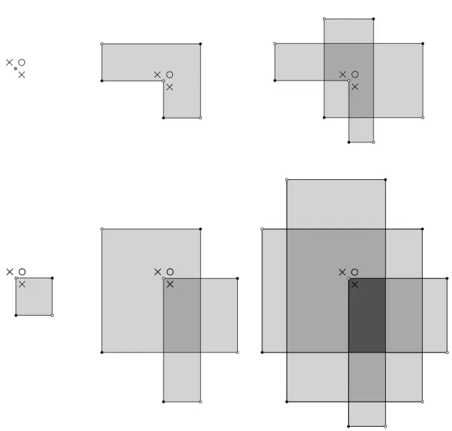
Definition 4.8. For grid statesx∈S(G0) andy∈I(G0) a positive domainp∈π(x,y) is called into L or of typeiL, if it is trivial, or if it satisfies the following conditions:
• At each corner point inx∪y\ {c}at least three of the four adjoining squares have local multiplicity 0.
• Three of the four squares attaching at the corner point c have the same local multiplicity k, and at the southwest square meetingc the local multiplicity of pisk−1.
• The grid statey has 2k+ 1components that are not in x.
The set of domains of typeiL is denoted byπiL(x,y)(see Figure 4).
Definition 4.9. Analogously, for grid statesx∈S(G0)andy∈I(G0)a positive domainp∈π(x,y)is called into Ror of type iR, if it satisfies the following conditions:
• At each corner point inx∪y\ {c}at least three of the four adjoining squares have local multiplicity 0.
• Three of the four squares attaching at the corner point c have the same local multiplicity k, and at the southeast square meetingc the local multiplicity of pisk+ 1.
• The grid statey has 2k+ 2components that are not in x.
The set of domains of typeiR is denoted byπiR(x,y)(see Figure 4).
Figure 4. Destabilization domains of typeiL(first row) andiR (second row)
The domains of type iLandiR are calleddestabilization domains. We use the notationπD=πiL∪πiR.
Definition 4.10. Let the complexity of the trivial domain be one. For other destabilization domains the complexity tells the number of horizontal segments in the boundary of the domain.
For example the upper right domain on Figure 4 has complexity 5. Observe that the domains of typeiL are the destabilization domains with odd complexity, while the domains of type iR are the ones with even complexity.
Lemma 4.11. Let x,y ∈ S(G0) be grid states such that there exists a destabilization domain p∈ π(x,y) of complexity k. Then there is a sequence of grid states x1, ...,xk such that x1 = x, xk = y, and empty rectangles r1, ..., rk−1with ri ∈Rect◦(xi,xi+1), so thatpdecomposes asr1∗...∗rk−1. Among such rectangle sequences, there is a unique one in which every rectangle ri has an edge on the distinguished vertical circle going through c.
The proof of this lemma can be found as the proof of Lemma 13.3.11. in [10].
Now we are ready to introduce the chain map which gives the isomorphism between tGC−(G0) and tGC−(G) [[1−t]]⊕tGC−(G). For this, we will use the abbreviations ¯X := {X1, X3, ..., Xn} and ¯O :=
{O1, O3, ..., On}.
Definition 4.12.
TheRt-module homomorphismsDiL: tGC−(G0)→tGC−(G)[[1−t]]andDiR: tGC−(G0)→tGC−(G)are defined on a grid state x∈S(G)in the following way:
DiL(x) := X
y∈I(G0)
X
p∈πiL(x,y)
Ut·|X¯∩p|+(2−t)·|O¯∩p|·e(y)
DiR(x) := X
y∈I(G0)
X
p∈πiR(x,y)
Ut·|X¯∩p|+(2−t)·|O¯∩p|·e(y)
Proposition 4.13. DiL increases the grading by (1−t), whereasDiR preserves the grading.
Proof. Letx,y∈S(G0). First observe that grt(e(y)) = grt(y) + 1−t. To get the result aboutDiL, our goal is to show that forp∈πiL(x,y)
grt(x) = grt(Ut·|X∩p|+(2−t)·|¯ O∩p|¯ ·y).
Suppose that the complexity ofpisk∈N. Then by Lemma 4.11,pcan be decomposed as the juxtaposition of k−1 rectangles. Consider the Maslov and the Alexander gradings. From Equations (1) and (2) we have that
M(x)−M(y) = (1−2· |O∩r1|) + (1−2· |O∩r2|) +...+ (1−2· |O∩rk−1|) =
=k−1−2· |O∩p|=−2· |O¯ ∩p|,
A(x)−A(y) =|X∩p| − |O∩p|=|X¯∩p| − |O¯ ∩p|
because aniL-type domain containsO1 andX2with the same multiplicity.
grt(x)−grt(y) = (M(x)−M(y))−t·(A(x)−A(y)) =−t· |X¯ ∩p| −(2−t)· |O¯ ∩p|, from which we get
grt(x) = grt(Ut·|X¯∩p|+(2−t)·|O¯∩p|·e(y))−1 +t.
Now letp∈πiR(x,y) with complexityk.
M(x)−M(y) =k−1−2· |O∩p|= 1−2· |O¯ ∩p|, A(x)−A(y) =|X∩p| − |O∩p|=|X¯∩p| − |O¯ ∩p|+ 1
because in aniR-type domain the multiplicity ofX2 is one greater than the multiplicity ofO1. grt(x)−grt(y) = (M(x)−M(y))−t·(A(x)−A(y)) = 1−t−t· |X¯ ∩p| −(2−t)· |O¯ ∩p|, from which we get
grt(x) = grt(Ut·|¯X∩p|+(2−t)·|O¯∩p|·e(y)).
LetC:=tGC−(G)[[1−t]]⊕tGC−(G), and consider the map∂:C→Csuch that∂(x, y) = (∂t−(x), ∂t−(y)) holds for any (x, y)∈C. Obviously, the pair (C, ∂) is a chain complex.
Definition 4.14.
Let D:tGC−(G0)→C be the destabilization map defined for any x∈tGC−(G0)as D(x) := (DiL(x), DiR(y))∈C.
The map DiL can be decomposed asDiL =DiL1 +D>1iL, where the subscript indicates the restriction on the complexity of the destabilization domains. Using this, we can draw the following schematic picture for D, where the top row representstGC−(G0) with its decomposition asI⊕N, and the bottom row showsC.
The mapD can be seen in the arrows connecting the two rows.
I - N
tGC−(G)[[1−t]]
DiL1
? D
iL>1
⊕ tGC−(G) DiR
?
Proposition 4.15. The destabilization mapD is a chain map.
The proof of this proposition is based on counting regions on the grid diagram, and it is analogous to the proof of Lemma 13.3.13. in [10].
Proposition 4.16. Suppose that C and Ce are graded chain complexes over Rt, such that they are free modules, and the grades appearing in them is bounded above. Let α∈R≥0 andf :C→Ce be a graded chain map. Thenf is a quasi-isomorphism if and only if it induces a quasi-isomorphismf¯:C
Uα·C→Ce
Uα·Ce. Proof. Let (C, ∂) and (C0, ∂0) be two chain complexes overRt. Themapping coneof a chain mapf :C→C0 is the chain complex Cone(f) = (C⊕C0, ∂Cone), where the differential∂Cone for an element (c, c0)∈C⊕C0 is defined as
∂Cone(c, c0) = (−∂(c), ∂(c0) +f(c)).
Observe that Cone(f)
Uα·Cone(f)∼= Cone( ¯f).
Lemma 4.17. For C, C0 chain complexes, a chain map f :C→C0 is a quasi-isomorphism if and only if H(Cone(f)) = 0.
For the proof of this lemma see [10, Appendix A, Corollary A.3.3.].
Lemma 4.18. Suppose thatCis a free, graded chain complex overRtthat is bounded above. ThenH(C)6= 0 if and only if H
CUα·C
6= 0 for a fixedα∈R>0.
Proof of Lemma 4.18. We assumed that Cis free, thus there exists a short exact sequence
0 - C ·Uα
- C - C
Uα·C - 0
Considering the associated long exact sequence, it is easy to see that if H(C) = 0, thenHC Uα·C
= 0.
Now suppose that H(C)6= 0. Since C is bounded above, H(C) has a homogeneous, non-zero elementx with maximal grading. Then, xcannot be of the formy·Uα for any y∈H(C). Therefore xmust inject to H
CUα·C
, and this way we got a non-zero element ofH
CUα·C
.
From Lemma 4.17 we know that the mapfis a quasi-isomorphism if and only ifH(Cone(f)) = 0. According to Lemma 4.18, this is equivalent to H
Cone(f)
Uα·Cone(f)
6= 0. By our observation, this holds if and only ifH(Cone( ¯f)) = 0, which, by Lemma 4.17 again, is equivalent to ¯f being a quasi-isomorphism.
Now let us use the following notations.
C1:=tGC−(G0) and D1:=tGC−(G)⊕tGC−(G) [[1−t]], C2:=C1Ut·C1 and D2:=D1Ut·D1,
C3:=C2U2−t·C2 and D3:=D2U2−t·D2.
Furthermore, define f = D : C1 → D1 and let ¯f : C2 → D2 be the map induced by f. Finally, define
¯¯
f : C3 → D3, the map induced by ¯f. Apply Proposition 4.16 for α = 2−t. Then we get that if f¯¯is a quasi-isomorphism, then ¯f is also a quasi-isomorphism. Now apply Proposition 4.16 again, to have that if ¯f is a quasi-isomorphism, then f is also a quasi-isomorphism. To prove the stabilization invariance, we need to verify that f =D is a quasi-isomorphism. For this, it is enough to show that f¯¯is a quasi-isomorphism betweenC3andD3.
Definition 4.19. The fully blocked grid chain complexGCg(G) associated to the grid diagram Gis a free F2-module generated by the grid states ofGwith the differential
∂˜O,X(x) = X
yS(G)
X
{r∈Rect◦(x,y)|r∩O=r∩X=∅}
y.
Proposition 4.20. f¯¯is a quasi-isomorphism.
Proof. Recall the notion of the fully blocked grid homology ([10]), which is the simplest version of grid homology.
Observe thatC3∼=GC(g G0) andD3∼=GC(g G)⊕GC(g G)[[1−t]]. From the proof of [10, Proposition 5.2.2], it follows that there is a quasi-isomorphism fromC3toD3, which is in factf¯¯.
5. The knot invariant Υ
5.1. The definition ofΥ. LetM be a module overRt. The torsion submodule Tors(M) ofM is Tors(M) ={m∈M | there is a non−zerop∈ Rtwithp·m= 0}.
Definition 5.1. Fort∈[1,2],
ΥG(t) := max{grt(x)|x∈tGH−(G), xis homogeneous and non−torsion}
Theorem 5.2. Let GandG0 be two grid diagrams such thatG0 can be obtained from Gby a grid move. If t∈[1,2], thenΥG(t) = ΥG0(t).
Proof. If G0 can be obtained from G by a commutation, then from Theorem 4.1 we know that tGH− is invariant under commutation, thus ΥG(t) = ΥG0(t).
Suppose that G0 can be obtained from Gby a stabilization, and let d denote the maximal grade which appears among homogeneous non-torsion elements of tGH−(G). Then the maximal grade of homogeneous non-torsion elements oftGH−(G)[[1−t]]isd+ 1−t. In case oft∈[1,2],d+ 1−t≤d, thus the maximal grade of homogeneous non-torsion elements oftGH−(G0)∼=tGH−(G)⊕tGH−(G)[[1−t]] is alsod.
In case oft∈[0,1] the above proof does not work, but the Υ invariant can be defined by extending it to t ∈[0,2] symmetrically. For t ∈[0,1], let ΥG(t) = ΥG(2−t). Obviously, ΥG(t) is also a knot invariant for t∈[0,1].
Consequently, for a knotKandt∈[0,2] we can define ΥK(t) by taking a grid diagramGrepresentingK:
ΥK(t) := ΥG(t).
According to Theorem 5.2, this is well-defined, and the following corollary is immediate:
Corollary 5.3. For t ∈ [1,2], ΥK(t) is a knot invariant, that is, if K1 and K2 are isotopic knots, then ΥK1(t) = ΥK2(t).
5.2. Crossing changes. In this section we examine how Υ changes under crossing changes.
LetK+ andK− be two knots which differ only in a crossing.
Proposition 5.4. There are Rt-module maps
C−:tGH−(K+)→tGH−(K−) and C+:tGH−(K−)→tGH−(K+)
whereC− is homogeneous and preserves the grading, and C+ is homogeneous of degree−2 +t.C−◦C+ and C+◦C− are both the multiplication by U2−t.
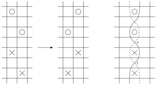
Before proving this proposition we introduce some notations: Represent the knotsK+andK− by the grid diagramsG+andG− differing by a cross-commutation of columns. Again, we draw these two diagrams onto the same torus so that theX- and theO-markings are fixed. Using the same notations as in Section 4.1, let α ={α1, ..., αn} be the horizontal circles of the diagrams, β ={β1, ..., βn} the vertical circles of G+, and γ={β1, ..., βi−1, γi, βi+1, ...βn}the vertical circles ofG−. Drawβiandγiso that they meet perpendicularly in four points, and these intersection points do not lie on any of the horizontal circles. This way the complement of βi ∪γi has five components, four of which are bigons marked by a single X or a single O. Label the O-markings so that O1 is above O2. Now the bigon marked by O2 has a common vertex with one of the X-marked bigons; denote this point bys. The twoX-labelled bigons share a vertex onβi∩γi, sinceG+can be obtained fromG− by a cross-commutation. Call this common pointt(Figure 5).
s
t
Figure 5. DrawingG+ andG− on the same torus, and the notation of the vertices
Proof of Proposition 5.4. Fix grid statesx+∈S(G+) andx− ∈S(G−). We use the notation Pent◦s(x+,x−) for the set of empty pentagons fromx+ tox− containingsas a vertex, and similarly, Pent◦t(x−,x+) for the set of empty pentagons fromx− to x+ with one vertex att.
Consider theRt-module maps c− :tGC−(G+)→tGC−(G−) andc+:tGC−(G−)→tGC−(G+) defined on a grid statex+∈S(G+) andx−∈S(G−) respectively in the following way:
c−(x+) = X
y−∈S(G−)
X
p∈Pent◦s(x+,y−)
Ut·|X∩p|+(2−t)·|O∩p|·y−
c+(x−) = X
y+∈S(G+)
X
p∈Pent◦t(x−,y+)
Ut·|X∩p|+(2−t)·|O∩p|·y+.
Lemma 5.5. The mapc− preserves thet-grading, whilec+ drops thet-grading by2−t.
Proof. The four marking between the circles βi andγi divide βi into four segments, call themA, B,C and Daccording to the followings: letAbe the segment between the twoO-markings, and from this part on, the order of the other segments to south isB,C andD. There is a natural one-to-one correspondence between