Gardener’s spline curve
Imre Juhász
Department of Descriptive Geometry, University of Miskolc agtji@uni-miskolc.hu
Submitted August 24, 2017 — Accepted November 29, 2017
Abstract
In the well-known gardener’s construction of the ellipse we replace the two foci by a finite set of points in the plane, that results in aG1spline curve that consists of elliptic arcs, if the set contains at least three non-collinear points. An algorithm is provided for the specification of these elliptic arcs, along with their control point based representation.
Keywords:Gardener’s construction, spline curve, rational Bézier representa- tion
MSC:65D17, 68U07
1. Introduction
A well-known way of drawing an ellipse is as follows. Place a piece of paper on the board, stick in two pins, loop a thread around the pins, pull taut with the tip of a pen and move the pen around, always keeping the loop of thread taut. As the pen moves around the two pins it will trace out an ellipse. This makes use of the fact that an ellipse is the locus of points, whose sum of distances from two fixed points is a constant. (Certainly, the usage of a thread is not a construction in the Euclidean sense.)
Replacing the paper by the ground, the pins by pegs, the thread with a string (or a rope) and the pen with a peg (or a spade), this procedure is used by gardeners to outline an elliptical flower bed. Therefore, this method is called the gardener’s construction (or the string method). It is not known when, where and by whom it has been invented but it is doubtless that this has been used by gardeners for quite a while.
http://ami.uni-eszterhazy.hu
109
A generalization of the gardener’s construction is attributed to Charles Graves, cf. [1], who replaced the two pins (the foci) by an ellipse and proved that the gardener’s construction results in another ellipse, confocal to the original one.
In what follows, we replace the two foci with a finite set of points in the plane, in which case the gardener’s construction produces a closedG1spline curve, which is composed of elliptic arcs. We provide an algorithm for the specification of the arcs, that enables us to draw this closed curve by means of a computer. This work was motivated by an incomplete, erroneous text (cf. [2]) found on the internet on a similar topic (its title is misleading).
2. Problem statement
If we loop a finite set of points in the plane (pins stuck in a board) with a string, pull taut with the tip of a pen and move the pen around, the string will always tighten on a part of the perimeter of the convex hull of the set. The convex hull of a finite set of points in the plane is always bounded by a closed convex polygon, the vertices of which are elements of the given set. There are several methods to compute the convex hull of a finite set of points, one can find them, e.g., in [3]
or [4].
If the set contains just a single point or all the points are collinear, the convex hull degenerates to a single point or to a straight line segment, respectively. In these degenerate cases the gardener’s construction produces a circle or an ellipse.
We exclude these trivial cases in our further study, i.e., we assume that the set contains at least three non-collinear points. From now on, we will examine closed convex planar polygons instead of a finite set of points.
Letp1,p2, . . . ,pnbe the vertices of a closed convex planar polygonP. Through- out the paper we make use of the convention
pi≡pimodn. (2.1)
This convention is applied for the half-lines and support lines as well, which will be introduced later. We assume that the orientation of the polygon is counter- clockwise. In what follows, if we list certain entities, like foci or delimiting lines, we always do it in the counterclockwise direction. The perimeter of the polygon is denoted byLp, i.e.,
Lp= Xn i=0
kpi+1−pik. Consider the distance L=Lp+δ, 0< δ∈R.
The support lines
li(t) = (1−t)pi+tpi+1, t∈R, i= 1,2, . . . , n
of sides of the polygon P divide the plane into 2nexternal parts (outside of the polygon), each part containing an arc of the closed curve. Each sidesi – bounded
by verticespiandpi+1– and each vertexpihas its own region that will contain an elliptic arc, that may degenerate to a single point in special circumstances. Side and vertex arcs alternately follow each other, the sequence is si,vi+1,(i= 1,2, . . . , n).
Each arc is a part of an ellipse, since the construction inherently ensures that the sum of the distances of any point of the arc from two certain vertices of the polygon is constant. Certainly, these two points (the foci) and the constant (the length of the major axis) vary arc by arc.
3. Triangle
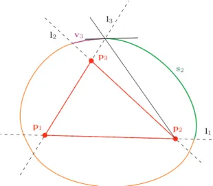
At first we consider the simplest case, the triangle. In this case we have the sequence of arcs si,vi+1,(i= 1,2,3). Foci of the side arcsi are pi,pi+1 and its endpoints are on support lines li−1,li+1 that we will refer to as delimiters of the arc. The vertex arcvihas the focipi−1,pi+2, and its delimiters areli,li−1. Consecutive arcs share a focus and a delimiter, moreover, at the common point of the two arcs the tangent lines are also coinciding, cf. Fig. 1. Thus, the result is aG1 spline curve that consists of elliptic arcs.
Figure 1: The case of the triangle: side arcs2 has the focip2,p3
and delimiters l1,l3; the consecutive vertex arc v3 has focip2,p1
and delimitersl3,l2. The two arcs have a common tangent line at their joint.
In the case of the triangle and the parallelogram, i.e., when support lines meet only at vertices of the polygon, this simple structure always works. Otherwise, ifδ is big enough, the determination of foci and delimiters of arcs may become much more complicated. Therefore, we have to construct an algorithm which can cope with any convex polygon.
4. Generic case
Our objective is to determine the defining data of consecutive elliptic arcs, i.e., the two foci, the delimiters of the arc and the length of the major axis, for any configuration of closed convex polygons. To this end, we introduce half-lines
hi(t) = (1−t)pi+tpi+1, 0≤t∈R, (1,2, . . . , n)
and build an intersection matrixMof sizen×n. Rows of this matrix correspond to half-lineshiand its columns to support lines lj. We examine only those intersection points of half-lines and support lines which differ from the vertices of the polygon.
Entry mi,j of matrix M equals 1 if the support line lj,(j > i+ 1) intersects the half-linehiand for the intersection point qij inequality
Lp−
j−1
X
k=i+1
kpk+1−pkk+kqij−pi+1k+kqij−pjk< L
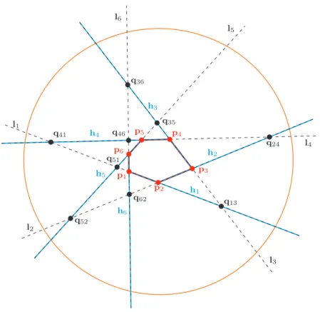
holds, otherwise mi,j = 0. Thus, the intersection matrix depends not only on the location of the vertices but onδas well. If in the above expression we have equality, it means that the arc is degenerated to a single point, which does not need any further study. The first support line (if there is any) that intersects the half-line hi has to beli+2 and if there are more than one such support lines, they must be consecutive ones, since the polygon is convex. (Note, that vertices, half-lines and support lines are cyclically arranged, convention (2.1) is used.) The intersection matrix of the configuration in Fig. 2 is
M=
0 0 1 0 0 0 0 0 0 1 0 0 0 0 0 0 1 1 1 0 0 0 0 1 1 1 0 0 0 0 0 1 0 0 0 0
.
Subsequently we provide algorithms for the specification of the list of foci and delimiters of the elliptic arcs, by processing the intersection matrix.
4.1. Specification of foci
In this subsection we produce the pair of foci of consecutive elliptic arcs by pro- cessing the intersection matrix row by row. Rows and columns of the intersection matrix can be considered as cycles, that is any element has a predecessor and a sub- sequent element according to the convention (2.1). We always process the vertices in counterclockwise direction. If in a list or in a sum the lower limitr` happens to be greater than the upper limitru, then the sequencer`, r`+ 1, . . . , n, n+ 1, ru is meant.
We process the intersection matrix row by row. Processing theith row of the intersection matrix(i= 1,2, . . . , n)is as follows.
Figure 2: Support lines li, half-lines hi (i= 1,2, . . . ,6) and the intersectionqij of halflines and support lines of a hexagon.
1. If mi,j= 0,(j = 1,2, . . . , n)then the pairs of foci are 1.1. ifmi−1,i+1= 0 then insertpi,pi+1
1.2. ifmi−1,i+2= 0 then insertpi,pi+2
2. Otherwise, find the first element k1 of the row which equals1 and the cor- responding entry in the previous row is0, i.e., mi,k1= 1 and mi−1,k1= 0, moreover findk2 which is the last element of the ith row of this property.
(The search always starts at columnj =i+ 1and goes around.) If there is no column that fulfills both requirements, then setk1= 0and findk` which is the last column containing1(regardless of the previous row). The pairs of foci are as follows.
2.1. Ifk1>0then
2.1.1. if the previous row is the zero vector, i.e.,mi−1,j= 0,(i= 1,2, . . . , n)then insertpi,pk1−1
2.1.2. insertpi,pk1; pi,pk1+1; . . . ,pi,pk2+1
2.2. else insertpi,pk`+1
The pairs of foci of the configuration in Fig. 2 are
1 1 2 2 3 3 3 4 4 5 5 6 3 4 4 5 5 6 1 1 2 2 3 3
.
4.2. Specification of delimiters
We specify the delimiters of consecutive elliptic arcs based on the intersection matrix. Consecutive pairs of the delimiters share an element, namely the second element of the current pair is the first element of the next one.
Processing of theith row of the intersection matrix is as follows.
1. If mi,j= 0,(j = 1,2, . . . , n),i.e., the row is the zero vector, then 1.1. ifmi−1,i+1= 0 then insertli−1,li+1; li+1,li
1.2. else insertli−1,li
2. Otherwise find the first element k1 of the row which equals 1 and the cor- responding entry in the previous row is0, i.e., mi,k1= 1 and mi−1,k1= 0, moreover find k2 which is the last column of the ith row of this property.
(The search always starts at columnj=i+ 1and goes round.) If there is no column that fulfills both requirements, then setk1 = 0. Pairs of delimiters are:
3. If k1>0then
3.1. if the previous row is the zero vector, then insert li−1,lk1−1;lk1−1,lk1; lk1,lk1+1;lk1+1,lk1+2;. . .;lk2−1,lk2
3.2. else insertli−1,lk1; lk1,lk1+1;lk1+1,lk1+2;. . .;lk2−1,lk2
3.3. insertlk2,li
4. else insert li−1,li
The delimiters of elliptic arcs of the configuration in Fig. 2 are 6 3 1 4 2 5 6 3 1 4 2 5
3 1 4 2 5 6 3 1 4 2 5 6
.
4.3. The length of the major axis
The length of the major axis of the ellipse defined by foci pi,pj (the order does matter) is
δ+
j−1
X
k=i
kpk+1−pkk.
5. Control point based representation
The best way for the description of elliptic arcs seems to be the quadratic rational Bézier form
X2 i=0
bi
wiBi2(t) P2
j=0wjB2j(t), t∈[0,1], (5.1) whereBi2(t),(i= 0,1,2)denote quadratic Bernstein polynomials, andwiare non- negative weights, such that w0+w1+w2>0. The three control points can easily be computed, since we know the two endpoints and the tangent lines there. If we use the standard form for the specification of the weights (w0 =w2 = 1) just the weight of the middle control point, i.e., w1 has to be computed which is also a routine exercise.
An alternative representation could be the trigonometric one (cf. [5]) X2
i=0
Aα2,i(t)bi, t∈[0, α], (5.2) where
Aα2,0(t) = 1
sin2 α2sin2 α−t
2
, Aα2,1(t) =2 cos α2
sin2 α2 sin α−t
2
sin t
2
, Aα2,2(t) = sin2 t2
sin2 α2.
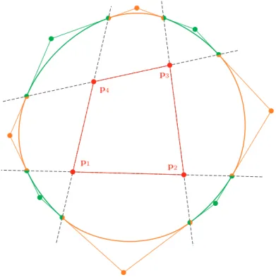
Its control pointsbi. (i= 0,1,2)coincide with that of (5.1), only shape parameter αhas to be calculated. Actually, (5.2) is just a reparametrization of (5.1). We prefer the rational Bézier representation. Fig. 3 shows the rational Bézier representation of the gardener’s spline curve for a quadrilateral.
If we use the standard form of weights for all elliptic arcsei,(i= 1,2, . . . ,2n) then we obtain aG1description of the gardener’s spline curve. In what follows we show a method for the C1 description of the curve that will be achieved by the transformation of weights.
Let us consider two consecutive arcs ei(t) =
X2 j=0
bi,j
wi,jB2j(t) P2
k=0wi,kB2k(t), t∈[0,1]
and
ei+1(t) = X2 j=0
bi+1,j
wi+1,jBj2(t) P2
k=0wi+1,kBk2(t),t∈[0,1].
Figure 3: The gardener’s spline curve of a quadrilateral, along with the control polygon of each quadratic Bézier curve that describe
the elliptic arcs, from which the curve is composed of
ForC1 continuity conditions
ei(t)|t=1= ei+1(t)|t=0, d
dtei(t)
t=1
= d
dtei+1(t)
t=0
have to be fulfilled. The first equality is guaranteed by the construction, only the second condition needs further study. Since
d dtei(t)
t=1
= 2wi,1
wi,2
(bi,2−bi,1), d
dtei+1(t)
t=0= 2wi+1,1
wi+1,0
(bi+1,1−bi+1,0) the equality
wi,1
wi,2
(bi,2−bi,1) =wi+1,1
wi+1,0
(bi+1,1−bi+1,0) (5.3)
has to be fulfilled for i = 1,2, . . . ,2n. If we have the standard form of weights, wi,2=wi+1,0= 1,(i= 1,2, . . . ,2n)this equality will not hold in general.
We will apply a suitable projective transformation of these standard weights (cf. [6]), which is equivalent to a linear fractional transformation of the parameter.
Thus we perform substitutions
wi,0→α2i, wi,1→αiwi,1, wi,2→1,
where αi, (i= 1,2, . . . ,2n) are positive real values to be determined. Applying these substitutions in Eq. (5.3), we obtain equalities
αiwi,1(bi,2−bi,1) = wi+1,1
αi+1 (bi+1,1−bi+1,0), (i= 1,2, . . . ,2n) which results in the system of equations
αiαi+1=βi,i+1, (i= 1,2, . . . ,2n) (5.4)
for the unknowns αi,(i= 1,2, . . . ,2n), where the positive constants βi,i+1 are of the form
βi,i+1=wi+1,1kbi+1,1−bi+1,0k
wi,1kbi,2−bi,1k , (i= 1,2, . . . ,2n). The solution is
α2= 1 α1
β1,2, α3=α1β2,3
β1,2
, ...
α2n= 1 α1
β1,2β3,4· · ·β2n−1,2n
β2,3β4,5· · ·β2n−2,2n−1, α1=α1β2,3β4,5· · ·β2n−2,2n−1β2n,1
β1,2β3,4· · ·β2n−1,2n , that is for the closed curve we have a solution if
β2,3β4,5· · ·β2n−2,2n−1β2n,1
β1,2β3,4· · ·β2n−1,2n
= 1
which is a very serious restriction. However, if we do not require C1 joint of arcs e1 ande2n, i.e., if we discard equation
α2nα1=β2n,1, we always have solutions, whereα1 is a free parameter.
References
[1] Glaeser, G., Stachel, H., Odehnal, B., The Universe of Conics: From the ancient Greeks to 21st century developments, Springer, 2016.
[2] Khilji, M. J., Thatipur, D. G., Multi foci closed curves,Journal of Theoretics 6.
[3] O’Rourke, J., Computational Geometry in C, 2nd Edition, Cambridge University Press, 1998.
[4] de Berg, M., Cheong, O., van Kreveld, M., Overmars, M., Computational Geometry: Algorithms and Applications, 3rd Edition, Springer, 2008.
[5] Sánchez-Reyes, J., Harmonic rational Bézier curves, p-Bézier curves and trigono- metric polynomials,Computer Aided Geometric Design, Vol. 15(1998) (9), 909–923.
[6] Patterson, R. R., Projective transformations of the parameter of a Bernstein-Bézier curve,ACM Transactions on Graphics, Vol. 4(1985) (4), 276–290.