34(2007) pp. 51–59
http://www.ektf.hu/tanszek/matematika/ami
On the shape parameter and constrained modification of GB-spline curves ∗
Yajuan Li
a, Miklós Hoffmann
band Guozhao Wang
caSchool of Science, Hangzhou Dianzi University, Hangzhou, China
bDepartment of Mathematics, Károly Eszterházy College, Eger, Hungary
cDepartment of Mathematics, Zhejiang University, Hangzhou, China Submitted 25 April 2007; Accepted 10 October 2007
Abstract
GB-spline curves can be considered as the generalization of B-spline curve incorporating a shape parameter into the polynomial basis functions. The geometric effect of the alteration of the shape parameter is discussed in this paper, including constrained shape control of the curve.
Keywords: GB-spline curves, shape parameter, paths, shape control, con- strained modification
MSC:68U05
1. Introduction
Although B-spline curve still plays central role in computer aided geometric design, the recently developed generalizations of this curve are also in the forefront of research. The well-known result of this attempt is the NURBS curve (c.f. [9]), but this curve has rational coefficient functions, yielding computational stability problems. Some recently developed methods tried to incorporate shape parameters into the original, polynomial basis functions. One of the earliest methods in this way is β-spline curve with two global parameters ([1, 2]). Further methods have been provided by direct generalization of B-spline curves as αB-splines in [8] and [10] and recently as GB-splines in [3]. Some alternative spline curves with shape parameters can be found in [4, 5, 6].
∗Research supported by the Hungarian National Scientific Fund (OTKA No. T048523) and the National Office of Research and Technology (Project CHN-37/2005).
51
for trigonometric CB-spline curves in [7]. In Section 2 we study the paths obtained by altering the shape parameter of the curve, and prove that points of the curve move along straight line segments. Applying this fact in Section 5 linear blending is used for constrained shape control, where the shape parameter is modified in a way that the new GB-spline curve passes through a given point.
2. GB-spline curve and its λ -paths
In [3] the GB-spline curve as a generalization of the classical uniform cubic B- spline curve with shape parameter has been introduced. The definition of an arc of a GB-spline curve with shape parameterλis as follows.
Definition 2.1. Given a sequence of control pointsPi,(i= 0, . . . ,3)the arc of the GB-spline curve is
C(λ, t) =
3
X
i=0
Pibi(λ, t), λ∈[−8,∞), t∈[0,1], (2.1)
where the GB-spline basic functions are b0(λ, t) = 2
12 +λ(1−t)3 b1(λ, t) = 1
12 +λ 2 (3 +λ)t3−3 (4 +λ)t2+ 8 +λ
(2.2) b2(λ, t) = 1
12 +λ −2 (3 +λ)t3+ 3 (2 +λ)t2+ 6t+ 2 b3(λ, t) = 2
12 +λt3.
This arc can simply be extended to a multi-arc non-uniform cubic GB-spline curve in a usual way, using four consecutive control points and applying the substitution
t= u−ui ui+1−ui
at each arc, where u∈ [ui, ui+1). Since the shape parameter has the same effect on each arc, we will focus on the single arc (2.1) in this paper.
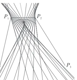
Now we consider the paths P(λ, t0) of the point C(t0) of the curve as the parameterλhas been changed. Note, that in these pathsλis the running parameter and t is the family parameter. Throughout this paper these paths are called λ- paths.
Theorem 2.2. The limit points of theλ-pathsP(λ, t0)atλ→ ∞are fixed points of the control legP1P2 and have symmetrical positions for the midpoint of the leg.
Figure 1: GB-spline curve and itsλ-paths
Proof. By simple calculation
λ→∞lim b0(λ, t) = lim
λ→∞b3(λ, t) = 0
λ→∞lim b1(λ, t) = 2t3−3t2+ 1
λ→∞lim b2(λ, t) =−2t3+ 3t2.
Denoting the latter limits byb1(∞, t)andb2(∞, t), and observing, thatb2(∞, t) = 1−b1(∞, t)it is obvious, that the limit points of the paths are
λ→∞lim P(λ, t) =L(t) =b1(∞, t)P1+ (1−b1(∞, t))P2 (2.3) while at t= 0.5we obtain0.5P1+ 0.5P2and this completes the proof.
Theorem 2.3. The λ-paths are straight line segments.
Proof. We prove that for any fixedt∈[0,1]the points of the pathP(λ, t)can be described as barycentric combination of the two endpointsP(−8, t)andP(∞, t) = limλ→∞P(λ, t). The blending functions atP(−8, t)are
b0(−8, t) = 1
2(1−t)3 b1(−8, t) = −5
2 t3+ 3t2 b2(−8, t) = 1
2(5t3−9t2+ 3t+ 1)
We can observe that
b0(λ, t)
b0(−8, t) = b3(λ, t)
b3(−8, t) = 4
12 +λ (2.4)
and denoting this quotiens byq(λ), after some calculation we obtain that b1(λ, t) =q(λ)b1(−8, t) + (1−q(λ))b1(∞, t)
b2(λ, t) =q(λ)b2(−8, t) + (1−q(λ))b2(∞, t), thus finally for any point of the path we get
P(λ, t) =q(λ)P(−8, t) + (1−q(λ))P(∞, t) (2.5)
and this was to be proved.
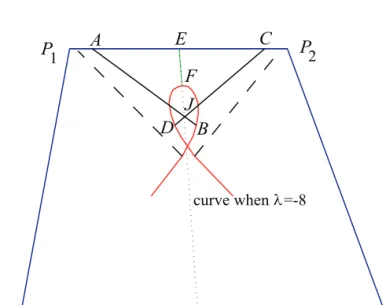
Theorem 2.4. Considering the symmetricλ-pathsP(λ, t0)andP(λ,1−t0), these lines may intersect each other. These intersection points are on the path of the point associated to the parameter valuet= 1/2, that is at the lineP(λ,1/2), if the lines P0P3 andP1P2 are parallel (see Fig. 2).
Figure 2: Symmetric paths intersect each other at a path associ- ated tot= 1/2
Proof. It is easy to prove that the shape of a GB-spline curve is independent of the choice of coordinates, i.e. (2.2) satisfies the following two equations:
C(λ, t, P0∗T+r, P1∗T+r, P2∗T+r, P3∗T+r)≡C(λ, t, P0, P1, P2, P3)∗T+r (2.6) where r is an arbitrary vector, and T is an arbitrary3×3 matrix. From above we know that the GB-spline curve, the symmetric lines and the midpoint of the segments are all preserved by an affine transformation, so we can prove the result in a special case using the coordinate system given in Fig. 2.
For arbitrary parametert, let the symmetric paths P(λ, t0) and P(λ,1−t0) intersect the control leg P1P2 and the curve C(−8, t) at the point A, B, C, D re- spectively, and the middle path corresponding tot= 0.5is on the line segmentEF withE, F are midpoints ofP0P3 andP1P2 respectively. Then using the definition of GB-spline curve, the coordinates of these points can be computed as follows:
A= ((3t2−2t3)a,1)
B = 1/2((5t3−9t2+ 3t+ 1)a+t3,1 + 3t−3t2) C= ((1−3t2+ 2t3)a,1)
D = 1/2((6t2−5t3)a+ (1−t)3,1 + 3t−3t2) E = (a/2,1)
F = (7/16a+ 1/16,7/8)
Thus we obtain the coordinates of intersection pointJ of the lineABandCD:
J =
(3t4−6t3−2t2+ 3t+ 1)a2+ (−3t4+ 6t3−3t2)a (9t2−9t−3)a+t2+ 1 , (6t4−12t3−4t2+ 10t+ 2)a+ (−t2+t−1)
(9t2−9t−3)a+t2+ 1
. (2.7)
To prove that the symmetric paths intersect each other at the path of the point associated to the parameter valuet= 0.5, we can prove that the pointJ is on the line segmentEF. The reciprocal of slope ofEF is
1 kEF
= a−1
2 (2.8)
Connecting the points EJ, the reciprocal of slope ofEJ is a−12 too. So the point J is located on the lineEF (or located on its extending part). That completes the
proof.
3. Passing through a given point
For practical applications, we would like to find a GB-spline curve passing through a given point among the family curves with the same control polygon. Of
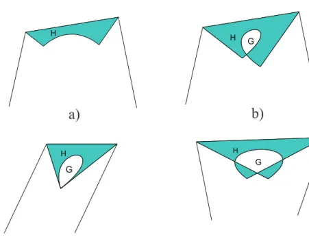
curve, the control leg P1P2 and the paths whenλ = 0,1 (See Fig. 3.a). If we let λ > −8 then the shape of the constrained region is a bit more complex. For a convex polygon, the region includes two parts in general. There is only one curve passing through a given point in one region, while there are two curves passing through a given point in another. Definitely, for every point in this region, we can find no less than one curve passing through it. By the property of the given convex control polygonPi, i= 0, . . . ,3, we can give the shape of the constrained region:
1) If two legsP0P1, P2P3 contend outside, the regionH ⊕G is circled by leg P1P2, paths whenλ= 0,1and the curve whenλ=−8as shown in Fig. 3. b.
2) When control polygon is a parallelogram, this regionH⊕Gis a triangle (See Fig. 3. c).
3) Otherwise this region is circled by legP1P2, paths when λ = 0,1 and the curve whenλ=−8as shown in Fig. 3. d.
Figure 3: Different cases of constrained region for shape control.
At each point in region H exactly one curve passes through, while in region G there are two solutions for each point.
Then for every point P in this region, we should find two parameter values λ0 and t0 for which C(λ0, t0) = P. As we have mentioned before, when λ < 0, the GB-spline curve is “below” the standard B-spline curve and in this case the variation diminishing property does not necessarily fulfilled. Thus in the following
we restrict ourselves for the case λ>0, however the described method works for λ <0as well.
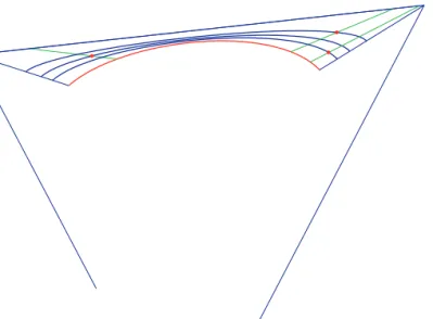
Figure 4: Given three points in the constrained region (λ>0) the shape parameter is modified in a way that the curves pass through
at the given points
We know that GB-spline paths are all lines, so we can find the value of t0 by the following dichotomy method.
Letf irst= 0, last= 1:
a) Lett∗= (f irst+last)/2 and compute two endpointsC(0, t∗)andC(∞, t∗) of path lineC(λ, t∗).
b) IfP is just on the path lineC(∞, t∗)within an allowed error, we gett0=t∗. The algorithm ends.
c) Otherwise we letlast=t∗(whenP andb0are on the same side of path line) or f irst=t∗ (whenP andb3 are on the same side of path line). Then we return to step a).
After obtaining the value of t0, we can get the value of λ0 by the following calculation. From (2.5) one can get
P(λ0, t0) =q(λ0)P(−8, t0) + (1−q(λ0))P(∞, t0) which yields
q(λ0) = P−P(∞, t0) P(−8, t0)−P(∞, t0)
for each coordinates of the pointsP, P(∞, t0)andP(−8, t0). Choosing for example
λ0=
Px−Px(∞, t0) −12.
By the above algorithm the curveC(λ0, t)passes through the given pointP at the parameter valuet0 (Fig. 4).
4. Conclusion and further research
GB-spline curves has been studied in the paper with special emphasis on the numerical and geometrical effects of the alteration of its shape parameter λ. The curve has also been described in a linear blending way, where a cubic blending function was used to combine the classical B-spline curve and its control polygon leg. This approach may worth for further examination to study other curves with shape parameters as linear blending curves to give an overall view and comparison of these curve types.
References
[1] Barsky, B.A. andBeatty, J.C., Local control of bias and tension inβ-splines, ACM Transactions on Graphics, 2 (1983) 109–134.
[2] Barsky, B.A., Computer graphics and geometric modeling using β−splines, Springer-Verlag, Berlin, 1988.
[3] Guo, Q., Cubic GB-spline curves,Journal of Information and Computational Sci- ence, 3 (2005) 465–471.
[4] Habib, Z., Sakai, M.andSarfraz, M., Interactive Shape Control with Rational Cubic Splines, International Journal of Computer-Aided Design & Applications, 1 (2004) 709–718.
[5] Habib, Z., Sarfraz, M.andSakai, M., Rational cubic spline interpolation with shape control,Computers & Graphics, 29 (2005) 594–605.
[6] Han, X., Piecewise quartic polynomial curves with a local shape parameter,Journal of Computational and Applied Mathematics, 195 (2006) 34–45.
[7] Hoffmann, M., Li, Y. andWang, G., Paths of C-Bézier and CB-spline curves, Computer Aided Geometric Design, 23 (2006) 463–475.
[8] Loe, K.F.,αB-spline: a linear singular blending spline,The Visual Computer, 12 (1996) 18–25.
[9] Piegl, L.andTiller, W., The NURBS book,Springer Verlag, Berlin, 1995.
[10] Tai, C.L.andWang, G.J., Interpolation with slackness and continuity control and convexity preservation using using singular blending,Journal of Computational and Applied Mathematics, 172 (2004) 337–361.
Yajuan Li
School of Science, Hangzhou Dianzi University, Hangzhou 310027, China Miklós Hoffmann
Department of Mathematics, Károly Eszterházy College, H-3300 Eger, Hungary Guzhao Wang
Institute of Computer Graphics and Image Processing, Department of Mathematics, Zhe- jiang University, Hangzhou 310027, China