Proceedings of the ASME 2020 International Design Engineering Technical Conferences &
Dynamic Systems and Control Conference DSCC 2020 October 4-7, 2020, Pittsburgh, USA
DSCC2020-3254
DRAFT: THE EFFECT OF TIME DELAY ON THE STABILITY CONTROL OF TRAILERS
Hanna Zs. Horvath∗ Department of Applied Mechanics
Budapest University of Technology and Economics Budapest, 1111
Hungary
Email: hanna.horvath@mm.bme.hu
Denes Takacs
MTA-BME Research Group on Dynamics of Machines and Vehicles
Budapest, 1111 Hungary takacs@mm.bme.hu
ABSTRACT
The instability of the car-trailer systems very often leads to the snaking and/or rocking motions of trailers. In order to reduce the safety risk of these unwanted vibrations, stability control can be applied. In this paper, we use a spatial trailer model to ana- lyze the effect of a possible control algorithm, which actuates by means of braking. For the sake of simplicity, the dynamics of the towing vehicle is modeled by the lateral displacement of the tow hitch that is supported laterally by a spring and damper. The lon- gitudinal speed of the vehicle is kept constant. The effect of the braking forces are emulated in our study via a control torque, which is proportional to the yaw angle and the yaw rate. The time delay of the controller is also considered. Linear stability charts are constructed in the plane of the different system pa- rameters. Linearly stable and unstable parameter domains are identified both for the vertical position of the center of gravity and the control gains. Numerical simulations are used to vali- date the theoretical results.
INTRODUCTION
The lateral stability problems of vehicles are in focus in the literature long time ago. Mechanical models with differ- ent complexity are constructed and widely used to analyze dif- ferent phenomena in vehicle dynamics. The shimmy motion of steered wheels [1, 2], wobble motion of motorbikes [3] and
snaking/rocking motion of trailers [4–7] are also current topics even nowadays.
Unfortunately, no universal solutions exist for the above mentioned vibration problems. Usually the geometrical param- eters that would be beneficial to avoid these vibrations are not optimal from other viewpoints. Thus, the development of stabil- ity control algorithms came to the forefront. Several studies in- vestigated active control methods [8–10] to improve the stability of vehicle-trailer combinations, but these are based on in-plane vehicle models. It is also shown in this study, that the linear sta- bility of the straight motion of the trailer is not affected by the pitch motion of the trailer. But a recent result [11] identified a relevant effect on local bifurcations at the stability boundaries.
In this paper, the stability of trailers is analyzed via a spatial four degree-of-freedom mechanical model. All the yaw, pitch and roll motions of the trailer are considered, while the motion of the towing car is imitated by the lateral displacement of the king pin. The model was already used in [11], where the nonlinear vibrations were investigated also taking into account the non- smooth nature of the tire characteristics.
Here, we focus on the linear stability only, but we try to give some hints about the effect of a possible stability control algorithm. A linear feedback control is used to enhance the sta- bility properties of the straight line motion of the trailer. For- mer studies often use similar or more sophisticated control algo- rithms, but suppose that the sampling time of the implemented electronic units is small, and the effect of the caused time delay
is negligible. If the stability control is based on conventional in- ertial sensors (e.g. accelerometers), this assumption can be valid.
When the stability control is based on the new features of an au- tonomous vehicle (e.g. GPS localization and image processing), the sensor systems can have more relevant time delay although the performance of stability control can be better, see [12]. In our study, this increased time delay of the controller is taken into account, and linear stability charts are constructed ot check its effect on the stability.
The contents of the paper is the following. First, the me- chanical model of the trailer is introduced. Then the system is linearised about the straight line motion, for which we also present the equations of motion. Linear stability charts are pre- sented in the plane of the parameters of trailer and the controller.
For a specific parameter setup, the effect of the time delay is also shown. Finally, numerical simulation results are presented.
MECHANICAL MODEL
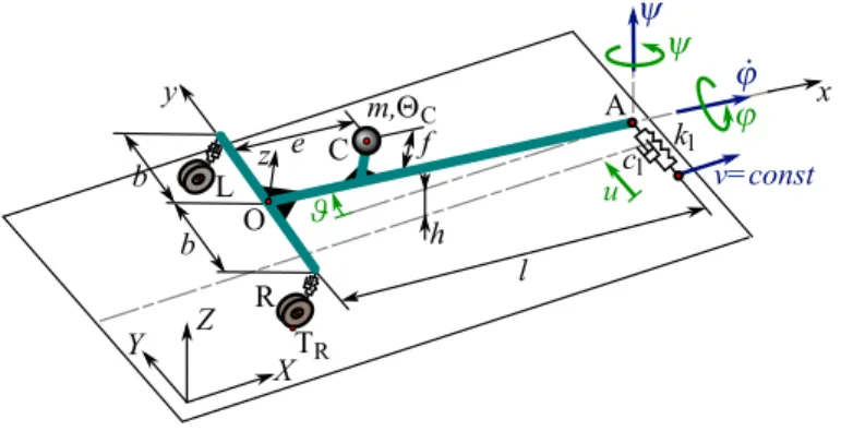
The spatial, 4 degrees-of-freedom (DoF) mechanical model of towed two-wheeled trailers is shown in Fig. 1. Two coordinate systems are differentiated: the ground-fixed coordinate system is denoted by(X,Y,Z), while the(x,y,z)coordinate system is fixed to the trailer itself.
X Y Z
C f
v=const e
m, C
L O
R TR b
b l
A
h
u
y x
z kl
cl
FIGURE 1. THE MECHANICAL MODEL OF TOWED TWO- WHEELED TRAILERS.
The trailer is towed at the king pin A with a constant longi- tudinal speedv. The mass and the mass moment of inertia is de- noted bymandJC, respectively. The center of mass is positioned at point C, its horizontal and vertical position can be described with parameterseand f. The vertical distance between the king pin A and the ground ish, the track width is 2band the caster length isl. Points R and L are the center points of the right and the left wheels, respectively. The contact points between the tires and the ground are marked by TRand TL. The stiffness and the
damping of the wheel suspensions and the tires are taken into ac- count as an overall stiffnesskand an overall dampingc. A spring of stiffnesskl and damper of dampingclare applied to support laterally the king pin at point A, as a representation of the effect of the towing vehicle.
The motion of the trailer can be described with the yaw an- gleψ(t), the pitch angleϑ(t), the roll angleϕ(t)and the lateral displacement of the king pinu(t). Thus the system hasn=4 degrees of freedom, the vector of the generalized coordinates is
q(t) =
ψ(t)ϑ(t)ϕ(t)u(t)T
. (1)
GOVERNING EQUATIONS
Since the system is holonomic, that is there are only geo- metrical constraints, the equations of motion can be derived with the Lagrange equation of the second kind [13]. For details of the derivation of the governing equations, see [11]. Here, we ex- tend the model of [11] by the effect of the braking forces that are generated by the stability control.
The active forces acting on the trailer are shown in Fig. 2, whereGis the gravitational force;FRtyre andFLtyre are the tire forces acting at points TR and TL;FRsusp andFLsusp are the sus- pension forces acting on the chassis of the trailer at points R and L; FAlat is the lateral force acting at point A;FRbrake andFLbrake are the braking forces.
Z X Y L C
R
A G
x y
z
FR tyre,lat
TR
FR tyre,z
FR susp
v=const FA lat
FL tyre,lat FL tyre,z
FL susp TL
FR brake FL brake
FIGURE 2. THE ACTIVE FORCES ACTING ON THE TRAILER.
The magnitude of the lateral component of the tire forces can be calculated with the help of the so-called Pacejka’s Magic Formula [2]. The mass of the wheels is not taken into account, therefore the vertical load on the tires can be calculated from the suspension forces.
For the sake of simplicity, the effect of the braking forces is emulated in our study with the control momentMcacting in the zdirection, see Fig. 3. The use of this control moment does not consider all of the effect of the braking forces, namely it does
not influence the pitch motion of the trailer, and it neglects the non-smooth characteristics of the forces that would emerge in the equations of motion. The more precise consideration of these effects will be the tasks of future studies.
Z X Y L C
R
A G
x y
z
FR tyre,lat
TR
FR tyre,z
FR susp
v=const FA lat
FL tyre,lat
FL tyre,z
FL susp TL
Mc
FIGURE 3. THE ACTIVE FORCES ACTING ON THE TRAILER, WHERE THE BRAKING FORCES ARE EMULATED WITH CON- TROL MOMENTMc.
Thus, the control moment is based on the linear feedback:
Mc=
0 0 Mc
(x,y,z)
=
0 0
−Pψ(t−τ)−Dψ(t˙ −τ)
(x,y,z)
, (2)
whereτ is the time delay of the control system. The equations of motion can be linearised around the rectilinear motion which corresponds toq0=0, namely
ψ(t)≡ψ0=0, ϑ(t)≡ϑ0=0, ϕ(t)≡ϕ0=0, u(t)≡u0=0.
(3)
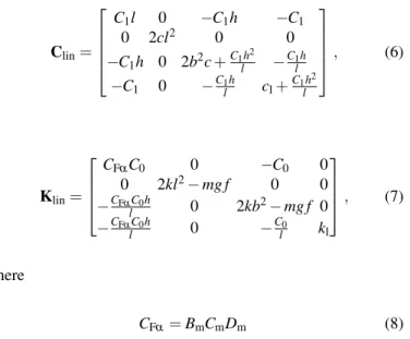
The linearised equations of motion can be written as Mlinq(t) +C¨ linq(t) +˙ Klinq(t) =Plinq(t−τ) +Dlinq(t˙ −τ), (4) whereMlinis the mass matrix, Clinis the damping matrix and Klinis the stiffness matrix of the linearised system:
Mlin=
JA,z 0 m f(l−e)−m(l−e)
0 JA,y 0 0
m f(l−e) 0 JA,x −m f
−m(l−e) 0 −m f m
, (5)
Clin=
C1l 0 −C1h −C1
0 2cl2 0 0
−C1h 0 2b2c+C1lh2 −C1lh
−C1 0 −C1lh cl+C1lh2
, (6)
Klin=
CFαC0 0 −C0 0
0 2kl2−mg f 0 0
−CFαlC0h 0 2kb2−mg f 0
−CFαlC0h 0 −Cl0 kl
, (7)
where
CFα=BmCmDm (8)
is the so-called cornering stiffness, whereBm,CmandDmare the stiffness, shape and peak factors of the Magic Formula. We also introduce
C0=mg(l−e) and C1=CFαC0
v (9)
in order to shorten the formulas. The matrices corresponding to the control moment are the following:
Plin=
−P0 0 0 0 0 0 0 0 0 0 0 0 0 0 0
, Dlin=
−D0 0 0 0 0 0 0 0 0 0 0 0 0 0 0
. (10)
As it can be seen, the linearised system can be separated into two subsystems: one differential equation can be disjointed, namely the pitch motion can be analyzed alone (1 DoF subsystem), while the remaining equations are coupled (3 DoF subsystem).
By using exponential trial function
q(t) =Aeλt (11) in Eqn. (4), we obtain:
Mlinλ2+Clinλ+Klin
Aeλt= (Plin+Dlinλ)Aeλ(t−τ). (12)
This can be rearranged as
Mlinλ2+Clinλ+Klin−(Plin+Dlinλ)eλ(−τ)
A=0. (13)
TABLE 1. PARAMETER VALUES OF THE TRAILER.
Notation Parameter Value
l caster length 3 m
b half of the track width 0.8 m h height of the king pin 0.5 m e horizontal position of CG 0.9 m f vertical position of CG 1 m
m mass of the trailer 3000 kg
k stiffness of the suspension 60 kN/m c damping of suspension 6 kNs/m
kl lateral stiffness 10 kN/m
cl lateral damping 100 Ns/m
Bm stiffness factor 10
Cm shape factor 1.9
Dm peak factor 1
Em curvature factor 0.97
The characteristic function of the system can be calculated as the determinant of the coefficient matrix, namely:
Dchar(λ):=det
Mlinλ2+Clinλ+Klin−(Plin+Dlinλ)eλ(−τ) (14) Due to the presence of the time delay, the characteristic equationDchar(λ) =0 is transcendental, but the stability bound- aries can be determined, where pure complex characteristic roots exist. Here, we use the D-subdivision method, namelyλ =iω is substituted into Eqn. (14) and the real and imaginary parts are separated:
Re(Dchar(iω)) =0,
Im(Dchar(iω)) =0. (15) In case of our system, the boundaries cannot be calculated analytically, but it can be analyzed numerically. The Eqns. (15) can be solved for example with the help of theMultidimensional Bisection Method[14] for a specific range of two system param- eters meantime the angular frequencyωis swept.
THE EFFECT OF TIME DELAY ON LINEAR STABILITY The effects of the stability control are investigated for a spe- cific parameter setup shown in Tab. 1. In Fig. 4, linear stability
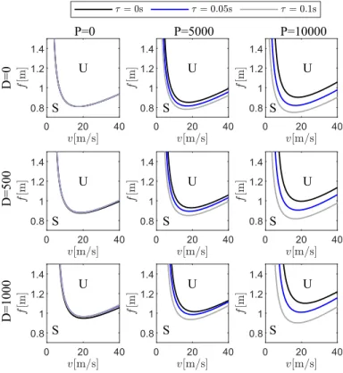
charts are plotted in the plane of the vertical position fof the cen- ter of gravity and the towing speed for different time delays. The panels of each figures are plotted for different PandDcontrol parameter values. The thick black, blue and grey lines corre- spond to the linear stability boundaries. The linearly stable (S) and unstable (U) regions are also marked.
For the case when there is no time delayτ=0 (see the con- tinuous black line in Fig. 4), it can be seen, the linearly unsta- ble region decreases when the values of the control gains are in- creased.
Having even small time delay in the systemτ=0.05 s, the linearly unstable region increases relative to the zero time de- lay case, see the continuous blue line in Fig. 4. But the use of the stability control is beneficial, namely linearly unstable region shrinks as the control gains are increased.
When the time delay is greater, namely whenτ=0.1 s is set, and the proportional gain P is increased, the linearly unstable region grows, see the grey line in Fig. 4. On the contrary, the increase of the derivative gain in the investigated parameter range remains advantageous with respect to the stability properties.
P=0 P=5000 P=10000
D=0D=500D=1000
U U U
U U U
U U U
S S S
S S S
S S S
FIGURE 4. THE STABILITY CHARTS FOR DIFFERENTPAND DCONTROL PARAMETER VALUES AND FORτ=0 s (BLACK LINE),τ=0.05 s (BLUE LINE) ANDτ=0.1 s (GREY LINE).
To analyze the stability of the control, one can also deter-
mine the critical values for the control gains for a specific setup of the trailer. Figure 5 shows the stability boundaries of the lin- earised system in the plane of the proportionalPand the deriva- tiveDgains forτ=0.1 s. In the figure, we use the parameters f =1 m andv=20 m/s. The stability boundary is plotted for ω ∈[0,100]rad/s. One can observe the static stability bound- ary (ω=0) at approximatelyP=−92000 Nm, see the vertical line in the figure. Below this proportional gain value a positive real characteristic root exists. To determine the stability prop- erties of the different regions of the stability chart one can use the semi-discretization [15], for example. This is a future task of our study. However, the stability properties can be checked with numerical simulations, too. In the figure, the light grey and white areas correspond to linearly unstable and stable domains, respectively.
S U
P1
FIGURE 5. THE STABILITY BOUNDARIES IN THE PLANE OF THE CONTROL GAINS FOR f=1 m,v=20 m/s ANDτ=0.1 s.
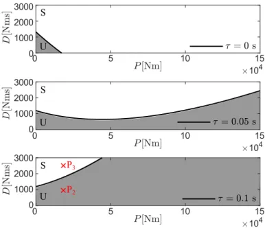
The stability charts can be shown for a more relevant con- trol parameter ranges, see Fig. 6. In the panels, the light grey and white areas correspond to linearly unstable and stable do- main, respectively. For the time delay free caseτ=0, the stabil- ity properties of the different regions were determined. For the non-zero delay case, we assume that the presence of a small time delay does not change the pattern of the stability regions. There- fore, the linearly stable and unstable domains are also shown for τ=0.05 s andτ=0.1 s, see the middle and bottom panel of Fig. 6. As can be seen, the linearly unstable domain is much greater in the examined region for larger time delay, as was ex- pected.
P3 U U
S S S
P2 U
FIGURE 6. THE STABILITY CHARTS FORτ=0 s, τ=0.05 s ANDτ=0.1 s.
NUMERICAL SIMULATIONS
The stability properties of certain points can be checked by means of numerical simulations. The equations of motion are rewritten in first order form:
q(t)˙
¨ q(t)
=
0 I
−Mlin−1Klin−Mlin−1Clin q(t)
˙ q(t)
+
0 0
Mlin−1PlinMlin−1Dlin
q(t−τ)
˙ q(t−τ)
,
(16)
which can be written as
˙
y(t) =Ay(t) +By(t−τ). (17) DDE23 was used with the initial condition y(t) =0 for t ∈ [−τ,0) and y(0) =
0 0 0 0Ω00 0 0T
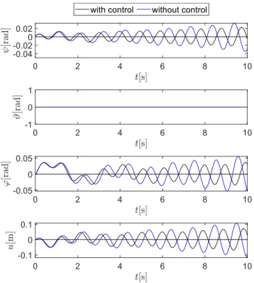
, where ˙ψ(0) =Ω0= 0.1 rad/s was applied as an impact-like perturbation. The time graphs of the generalized coordinates can be seen in Fig. 7, 8 and 9 for f =1 m, v=20 m/s and τ=0.1 s. In the figures ϑ(t)≡0 since the linearized governing equations are simulated in which the pitch motion is decoupled (see Eqn. (4)).
Static loss of stability can be seen in Fig. 7, which corre- sponds to parameter point P1in Fig. 5. That is, the trailer loses its stability without oscillations due to the fact that the system has a positive real characteristic root.
FIGURE 7. THE TIME GRAPHS OF THE GENERALIZED CO- ORDINATES FORτ=0.1 s,P=−100000 Nm ANDD=1000 Nms (STATIC LOSS OF STABILITY).
The trailer loses its stability via oscillations if the control gains areP=20000 Nm andD=1000 Nms, see the black con- tinuous lines in Fig. 8, which corresponds to parameter point P2 in Fig. 6. The oscillations without control can be seen with blue continuous lines. The effect of the impact-like initial perturba- tion in the yaw rate ˙ψ(t)excites all the vibration modes of the system that can be observed in the first half of the time graphs.
As can be seen, the oscillations are reduced by introducing the control.
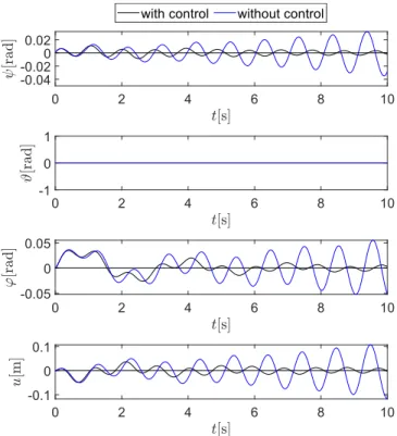
By increasing the value of the proportional gainPfor fixed D=1000 Nms, the motion becomes stable above a certain value.
An example for a stable motion is shown with black continuous lines in Fig. 9, which corresponds to parameter point P3in Fig. 6.
The oscillations without control can be seen with blue continuous lines. As can be seen, the otherwise unstable motion is stabilized with the help of the control.
CONCLUSIONS
A spatial model of two-wheeled trailers was introduced to analyze the stability of car-trailer systems. The effect of a pos- sible stability control was emulated by a control torque that is generated by the braking forces. Our approach only considers the effect of the control on the yaw dynamics, and do not take
FIGURE 8. THE TIME GRAPHS OF THE GENERALIZED CO- ORDINATES FORτ=0.1 s, WITH CONTROL (P=20000 Nm AND D=1000 Nms) AND WITHOUT CONTROL (DYNAMIC LOSS OF STABILITY).
into account the direct effect of the braking forces on the pitch motion. Moreover, in real case, the non-smooth characteristics of the braking forces can be relevant when the nonlinear oscillations are investigated.
However, some stability charts were shown and used to give some impression about the effect of the controller and the time delay. For a specific parameter setup, we showed that detailed analysis of the linear stability is necessary to determine the ap- propriate control gains when the time delay is large. More de- tailed and precise analysis is the task of our future work.
ACKNOWLEDGMENT
This research was partly supported by the National Re- search, Development and Innovation Office under grant no.
NKFI-128422 and by the Higher Education Excellence Program of the Ministry of Human Capacities in the frame of Artificial intelligence research area of Budapest University of Technology and Economics (BME FIKP-MI).
FIGURE 9. THE TIME GRAPHS OF THE GENERALIZED CO- ORDINATES FORτ=0.1 s, WITH CONTROL (P=20000 Nm AND D=2500 Nms) AND WITHOUT CONTROL (STABLE MOTION).
REFERENCES
[1] Schlippe, B., and Dietrich, R., 1941. “Das Flattern Eines Bepneuten Rades (Shimmying of a pneumatic wheel)”.
In Bericht 140 der Lilienthal-Gesellschaft f¨ur Luftfahrt- forschung, pp. 35–45, 63–66. English translation is avail- able inNACA Technical Memorandum 1365, pages 125- 166, 217-228, 1954.
[2] Pacejka, H., 2002. Tyre and Vehicle Dynamics. Elsevier Butterworth-Heinemann.
[3] Sharp, R. S., Evangelou, S., and Limebeer, D. J. N., 2004. “Advances in the modelling of motorcycle dynam- ics”.Multibody System Dynamics, 12(3), pp. 251–283.
[4] Troger, H., and Zeman, K., 1984. “A nonlinear-analysis of the generic types of loss of stability of the steady-state motion of a tractor-semitrailer”.Vehicle System Dynamics, 13(4), pp. 161–172.
[5] Darling, J., Tilley, D., and Gao, B., 2009. “An experimen- tal investigation of car–trailer high-speed stability”. Pro- ceedings of the Institution of Mechanical Engineers, Part D: Journal of Automobile Engineering, 223(4), pp. 471–
484.
[6] Beregi, S., Takacs, D., Gyebroszki, G., and Stepan, G., 2019. “Theoretical and experimental study on the nonlin-
ear dynamics of wheel-shimmy”.Nonlinear Dynamics, 98, pp. 2581–2593.
[7] Sharp, R. S., and Ferna´ndez, M. A. A., 2002. “Car-caravan snaking - part 1: the influence of pintle pin friction”. In Proceedings of the Institution of Mechanical Engineers Part C - Journal of Mechanical Engineering Science, Vol. 216 of 7, pp. 707–722.
[8] Hac, A., Fulk, D., and Chen, H., 2008. “Stability and con- trol considerations of vehicle-trailer combination”.SAE In- ternational.
[9] Kageyama, I., and Nagai, R., 1995. “Stabilization of pas- senger car-caravan combination using four wheel steering control”.Vehicle System Dynamics, 24(4-5), pp. 313–327.
[10] Deng, W., Lee, Y. H., and Tian, M., 2004. “An integrated chassis control for vehicle-trailer stability and handling per- formance”.SAE Technical Paper Series.
[11] Horvath, H. Z., and Takacs, D., 2020. “Analogue models of rocking suitcases and snaking trailers”. Nonlinear Dynam- ics of Structures, Systems and Devices, pp. 117–126.
[12] Olofsson, B., and Nielsen, L., 2020. “Using crash databases to predict effectiveness of new autonomous vehicle maneu- vers for lane-departure injury reduction”. IEEE Transac- tions on Intelligent Transportation Systems, pp. 1–12.
[13] Gantmacher, F., 1975. Lectures in analytical mechanics.
MIR Publishers, Moscow.
[14] Bachrathy, D., and Stepan, G., 2012. “Bisection method in higher dimensions and the efficiency number”. Periodica Polytechnica - Mechanical Engineering, 56(2), pp. 81–86.
[15] Insperger, T., and Stepan, G., 2011.Semi-Discretization for Time-Delay Systems. Springer New York, pp. 39–71.