Application of Predictor Feedback to Compensate Time Delays in Connected Cruise Control

(1)

Application of Predictor Feedback to Compensate Time Delays in Connected Cruise Control

Tamás G. Molnár, Wubing B. Qin, Tamás Insperger, and Gábor Orosz

Abstract— In this paper, we investigate a vehicular string traveling on a single lane, where vehicles use connected cruise control to regulate their longitudinal motion based on data received from other vehicles via wireless vehicle-to-vehicle com- munication. Assuming digital controllers, the sample-and-hold units introduce time-periodic time delays in the control loops and the delays increase when data packets are lost. We investigate the effect of packet losses on plant and string stability while varying the control gains and determine the minimum achievable time gap below which stability cannot be achieved. We propose two predictor feedback control strategies that overcome the destabilizing effect of the time delay caused by the sample-and- hold unit and packet losses.

Index Terms— Connected cruise control, predictive control, stability analysis, time delay.

I. INTRODUCTION

F

EEDBACK loops are always associated with certain time delays due to the finite speed of sensing, data processing, and actuation, and time delays are often considered to be the source of instability in dynamic systems. A promising way of stabilizing unstable time delay systems is the application of predictor feedback control strategies [1]. The main concept of predictor feedback is that the actual (delay-free) state of the system is predicted and used for feedback instead of the delayed state obtained from measurements or observers. The prediction can be based on the solution of an internal model of the dynamic system, which results in the so-called finite spectrum assignment (FSA) technique [2]–[5]. If the internal model is a perfect representation of the actual system, then the delay-free state can exactly be predicted, and a perfect implementation of the control law reduces the closed loop system to a delay-free system [2], [6]–[11]. This way, predictor feedback has the potential to stabilize systems with time delays.

Manuscript received January 12, 2017; revised April 4, 2017 and July 20, 2017; accepted September 15, 2017. Date of publication November 7, 2017; date of current version February 1, 2018. This work was supported by the U. S. National Science Foundation under Grant 1300319.

The Associate Editor for this paper was P. Zingaretti. (Corresponding author:

Tamás G. Molnár.)

T. G. Molnár is with the Department of Applied Mechanics, Budapest University of Technology and Economics, H-1111 Budapest, Hungary (e-mail:

molnar@mm.bme.hu).

W. B. Qin and G. Orosz are with the Department of Mechanical Engineer- ing, University of Michigan, Ann Arbor, MI 48109 USA (e-mail: wubing@

umich.edu; orosz@umich.edu).

T. Insperger is with the Department of Applied Mechanics, Budapest University of Technology and Economics, H-1111 Budapest, Hungary, and also with the MTA-BME Lendület Human Balancing Research Group, H-1111 Budapest, Hungary (e-mail: insperger@mm.bme.hu).

Color versions of one or more of the figures in this paper are available online at http://ieeexplore.ieee.org.

Digital Object Identifier 10.1109/TITS.2017.2754240

Time delays play a crucial role in the dynamics of vehicular traffic. In the case of human-driven vehicles, the reaction time of the driver – ranging between 0.3−1.5 [s] – is the most important source of time delay. This reaction time is often the source of instabilities in traffic flow and may lead to congestion or even cause accidents on the road. Since improving safety and mobility of vehicular traffic is a major concern today [12], advanced driver assistance systems (ADAS) were developed to overcome these problems. ADAS must satisfy two stability criteria with regards to the longitudinal dynamics of the vehicles. On one hand, plant stability must be guaranteed, which is associated with safe driving along a prescribed velocity profile. On the other hand, when a group of vehicles forms a vehicular string, congestion waves traveling upstream the traffic flow must be attenuated that is referred as string stability [13]. String instability typically leads to the formation of stop-and-go traffic jams [14], [15] that impacts mobility negatively.

Several strategies have been proposed in the literature to ensure plant and string stability. When using adaptive cruise control (ACC), the vehicle is equipped with radars or cameras to measure the distance headway and the velocity difference between the vehicle and the preceding vehicle [16]. The sensors used in ACC strategy may be supported (or substituted) by wireless vehicle-to-vehicle (V2V) communication that enables the vehicle to monitor the vehicle ahead even when it is beyond the line of sight. (Note that the headway and the velocity difference can also be calculated from GPS signals.) V2V communication may also improve the safety and mobility of traffic by providing information about multiple vehicles ahead [17], [18]. In cooperative adaptive cruise control (CACC), the members of a vehicular string are equipped with ACC, but also obtain information about the motion of a designated platoon leader using communication [19]–[21]. However, in real traffic situations, not all vehicles are equipped with range sensors and since the range of V2V communication is limited, the data about leader’s motion might not be accessible to every member of the vehicular string. Therefore, the concept of connected cruise control (CCC) was introduced in [18], [22], and [23], where all available V2V signals are utilized. This concept is applicable even in the presence of human-driven vehicles in the string and it can be used in realistic traffic scenarios. CCC can be used to support human drivers, to supplement sensory information, or to control the longitudinal motion of the vehicle.

In this paper, we investigate an application of the CCC concept while taking into account the intermittency in

See http://www.ieee.org/publications_standards/publications/rights/index.html for more information.

(2)

V2V communication. For example, dedicated short range communication (DSRC) devices typically use the sampling period 100[ms]to process the data during communication [24]–[26].

The sample-and-hold units used in digital controllers utilizing DSRC information introduce time-varying time delays into the control loop [27]. Disturbances during communication may lead to loss of data packets, which increases the time delay [28]. In this paper, we investigate the dynamics of vehicular strings when the communication is subject to deterministic packet loss scenarios. We investigate plant and string stability while varying the control gains for different numbers of consecutive packet losses and summarize our results using stability charts. We also show that the time delay gives a fundamental limit to the minimum achievable time gap, that is, to the maximum achievable flux in the traffic flow. The destabilizing effect of time delay on vehicle platoons was also demonstrated in [18], [23], and [27]–[32].

The main contributions of this paper are two predictor feedback control strategies that eliminate the destabilizing effect of the time-varying time delay. The first strategy estimates the velocity and the distance of the vehicles based on the last available data packets without requiring knowledge about the dynamics of the vehicular string. Such prediction can be done based on the history of GPS position and velocity contained by basic safety messages (BSM) [24]–[26]. The second strategy can be considered as an application of the FSA technique to a discrete-time system [4], [33]. This requires a dynamic model of the vehicles as the predicted state is obtained by the integration of the model. We show that the predictors may improve stability under intermittent communication and ensure robustness against the variations of time delay due to packet losses. Trade-off regarding using different predictors is also pointed out.

The outline of the paper is the following. Section II introduces the model of the vehicular string where the vehicles are driven by CCC. In Section III, we analyze the effects of the sample-and-hold units when digital controllers are used by members of the vehicular string. In Section IV, we carry out plant and string stability analysis. Section V demon- strates the effect of packet losses in wireless communication.

In Sections VI and VII, we introduce two predictor feedback control strategies to overcome the destabilizing effect of packet losses and to compensate the processing delay of the digital controller. Finally, we draw conclusions in Section VIII.

II. CONNECTEDCRUISECONTROL

In this paper, we consider a vehicular string on a single lane as shown in Fig. 1. We assume identical vehicles such that the motion of each member is controlled based on the position and velocity data received from the vehicle immediately ahead.

This way, the analysis of the vehicular string can be simplified to the analysis of the leader-follower configuration at the bottom of Fig. 1. The headway h, the leader’s velocity vL, and the follower’s velocityvF satisfy

h˙(t)=vL(t)−vF(t). (1) We assume that the follower’s acceleration can be adjusted directly by the controller:

˙

vF(t)=ades(t), (2)

Fig. 1. String of connected vehicles traveling on a single lane. The vehicular string can be considered as the concatenation of the leader-follower pattern shown below. The red dashed arrows indicate wireless vehicle-to-vehicle communication.

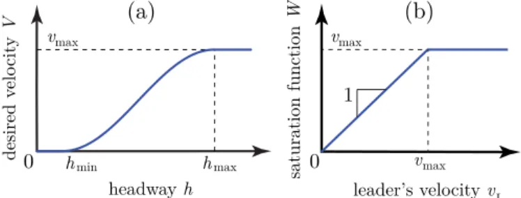
Fig. 2. (a) The desired velocity (4)-(5) as a function of the headway.

(b) The saturation function (6).

where ades(t)denotes the control input. We use a proportional- velocity (PV) controller widely used in the literature [18], [30]:

ades(t)=α V

h(t)

−vF(t) +β

W vL(t)

−vF(t) . (3) Hereαandβ denote the control gains, V(h)is the follower’s desired velocity that depends on the headway, and W(vL)is a saturation function. Note that several other control strategies also exist [22], [34]–[43] and the analysis carried out in this paper can also be applied to those controllers.

The controller (3) contains the range policy

V(h)=

⎧⎪

⎨

⎪⎩

0 if h≤hmin, F(h) if hmin<h<hmax, vmax if h≥hmax.

(4)

This states that the follower intends to stop if the headway drops below the limit hmin. Once the headway exceeds the limit hmax, the follower wants to travel with the maximum speed vmax allowed by road traffic regulations. Between these limits, the desired velocity increases monotonously according to the function F(h). We prescribe F(hmin)= 0, F(hmax)=vmax, F(hmin)=F(hmax)=0 in order to achieve smooth velocity and acceleration profiles. As an example, we satisfy these conditions by the choice

F(h)= vmax

2

1−cos

π h−hmin

hmax−hmin

, (5)

see Fig. 2(a). Note that any other monotonous and sufficiently smooth function F(h) could be used as well. Besides, other range policies also exist, see [23], [34], [44]–[46].

When the leader’s velocity exceeds the maximum speed vmax allowed by road traffic regulations, we switch off the connected cruise control. We realize this by the saturation

(3)

function

W(vL)=

vL ifvL≤vmax,

vmax ifvL> vmax, (6) that is displayed in Fig. 2(b).

From this point on, we assume vL ≤ vmax, where system (1), (2), (3) has a unique equilibrium

V(h^∗)=v^∗_F=v_L^∗. (7) This equilibrium represents the desired uniform flow, where each member of the vehicular string travels with the same constant velocity V(h^∗)while keeping a constant headway h^∗. The control gains α and β must be chosen such that we guarantee the stability of the equilibrium.

III. APPLICATION OF ADIGITALCONTROLLER

We assume that a digital controller is implemented to realize the control law (3), thus the headway h, the leader’s velocity vL, and the follower’s velocity vF are sampled with sampling period t. For dedicated short range com- munication (DSRC) devices, the typical sampling period is t=100[ms]. We assume that the clocks of the leader and the follower are synchronized, which can be achieved using satellites. Thus, all headway and velocity data is available at the same discrete time instants tk = kt. Note that it takes a certain amount of time for the leader to process the sensed data and to transmit it, and for the follower to receive data, to process it, and to use it for actuating the vehicle.

Therefore, at time instant tk, the controller is able to use the data measured at the previous sampling instant tk−1. This implies that the controller has a certain processing delay. The control input is held constant by a zero-order-hold (ZOH) unit along [tk,tk+1). Therefore, when a digital controller is implemented, the control law (2) modifies to

˙

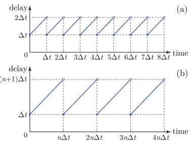
vF(t)=ades(tk−1), t∈ [tk,tk+1), (8) where ades is given by (3). Equations (1), (3), (8) define a continuous-time nonlinear system with piecewise constant input. Correspondingly, the processing delay introduced by the ZOH is time-periodic as shown in Fig. 3(a). During each sampling period, the time delay increases linearly from t, since ades(tk−1)is used at tk, to 2t, since ades(tk−1)is still used at tk+1. Note that since delayed states are available for the follower instead of actual ones, there is a possibility to improve control performance by estimating the actual state via predictors, which will be discussed further below.

According to [47], the dynamics (1), (3), (8) can be con- verted to a discrete-time map. In particular, we solve the system along t ∈ [tk,tk+1) with the initial conditions at tk, which gives

h(k+1) vF(k+1)

=

1 −t

0 1

h(k) vF(k)

+

−1 2αt² αt

V

h(k−1)

Fig. 3. The time delay caused by digital control: (a) without packet losses, (b) when every n-th packet is received.

+

0 1

2(α+β)t² 0 −(α+β)t

h(k−1) vF(k−1)

+ −1

2βt² βt

W

vL(k−1) +

tk+1

tk vL(t)dt 0

, (9) where h(k)=h(tk),vF(k)=vF(tk),vL(k)=vL(tk).

The stability of the uniform flow equilibrium (7) of system (1), (3), (8) is equivalent to the stability of the fixed point of the discrete-time map (9). Here, we restrict ourselves to linear analysis, therefore we linearize (9), which gives

h(k˜ +1)

˜

vF(k+1)

=

1 −t

0 1

h˜(k)

˜ vF(k)

+ −1

2αV(h^∗)t² 1

2(α+β)t² αV(h^∗)t −(α+β)t

h˜(k−1)

˜

vF(k−1)

+ −1

2βt² βt

˜

vL(k−1)+ t_k₊₁

t_k v˜L(t)dt 0

, (10) whereh˜(t),v˜L(t), andv˜F(t)denote small fluctuations around the equilibrium headway h^∗ and equilibrium velocity V(h^∗) given by (7). From (4), the derivative V(h^∗)reads

V(h^∗)=

⎧⎪

⎨

⎪⎩

0 ifh^∗≤hmin, F(h^∗) ifhmin<h^∗<hmax, 0 ifh^∗≥hmax.

(11) We assume sinusoidal fluctuations in leader’s velocity,

˜

vL(t)=v_L^ampsin(ωt), (12) since real fluctuations can be considered as an infinite sum of harmonic functions. This way, the integral in (10) can be written in the form

_t_k₊₁

t_k v˜L(t)dt=β0v˜L(tk)+β2v˜L(tk−2), (13)

(4)

where

β0= cos(2ωt)−cos(3ωt)

ωsin(2ωt) , β2=cos(ωt)−1 ωsin(2ωt). (14) If we define the state, the input, and the output of the linear system (10) as

x(k)= h˜(k)

˜ vF(k)

, u(k)= ˜vL(k), y(k)= ˜vF(k), (15) we can rewrite (10), (12) in the form

x(k+1)=a0x(k)+a1x(k−1)

+b0u(k)+b1u(k−1)+b2u(k−2),

y(k)=c x(k), (16)

where a0=

1 −t

0 1

, a1=

−1

2αV(h^∗)t² 1

2(α+β)t² αV(h^∗)t −(α+β)t

,

b0= β0

0

, b1= −1

2βt² βt

, b2=

β2

0

, c= 0 1

. (17) Now we introduce the augmented state vector

X(k)=

x(k) x(k−1)

, (18)

such that (16) is written in the state-space representation X(k+1)=A1X(k)+B0u(k)+B1u(k−1)+B2u(k−2),

y(k)=C1X(k). (19)

Here the system, the input, and the output matrices read A1 =

a0 a1

I 0

, B0= b0

o

, B1= b1

o

, B2= b2

o

, C1 =

c o^T

, (20)

where 0 ∈ R²^×² and I ∈ R²^×² are the zero and the identity matrices, respectively, o ∈ R² denotes the zero vector, and T stands for transpose.

IV. PLANT ANDSTRINGSTABILITY

When applying connected cruise control for vehicular strings, two stability criteria – plant and string stability – must be fulfilled. Plant stability is related to the safety and collision avoidance between vehicles, whereas string stability is associated with disturbance attenuation along vehicular strings and ensuring smooth traffic flow. We present the stability analysis of (19) in this section following the method shown in [27].

The system is plant stable if the follower is able to approach leader’s constant velocityv^∗_L. In the absence of fluctuations in the leader’s velocity (v˜L(t)≡0, u(k)=0), the linear map (19) simplifies to

X(k+1)=A1X(k). (21) Plant stability is guaranteed if all eigenvalues of A1lie within the unit circle in the complex plane. The eigenvalues are given by the characteristic equation

det(zI−A1)=0. (22)

Plant stability can be lost in three qualitatively different ways: an eigenvalue crosses the unit circle at 1, an eigenvalue crosses the unit circle at −1, a pair of complex conjugate eigenvalues crosses the unit circle. The first case leads to a non-oscillatory stability loss, while the last two lead to oscillatory stability loss. The corresponding plant stability boundaries are obtained for z =1, or z = −1, or z = e^±ⁱ^θ (i² = −1, θ ∈ (0, π)). Substituting z = 1 and z = −1 into (22) while using (17) and (20), we get the plant stability boundaries in the form

α=0, (23)

α= − 2

t −β, (24)

respectively. Substituting z = eⁱ^θ into (22) while using (17) and (20), and separating the real and the imaginary parts, we obtain the third plant stability boundary parameterized byθ∈(0, π):

α = 4 sin²θ+6 cosθ−6 V(h^∗)t² , β = 2 sin²θ+cosθ−1

t −4 sin²θ+6 cosθ−6

V(h^∗)t² . (25) Fig. 4(a) shows the plant stability boundaries in the plane (β, α). We used hmin = 5 [m], hmax = 35 [m], vmax=30[m/s] to define the range policy, and investigated the uniform flow equilibrium given by h^∗ = 20 [m], v_L^∗ = v_F^∗ = 15 [m/s], which imply V(h^∗) =π/2 [1/s]. We keep these parameters fixed throughout the paper. The dashed, the dotted, and the solid red lines correspond to the plant sta- bility boundaries associated with z=1, z= −1, and z=eⁱ^θ, respectively. They enclose the light gray-shaded plant stable domain. The eigenvalue plots in Fig 4(b) show the eigenvalues of matrix A1 for different plant stability losses (cases A, B, and C) and for a plant stable scenario (case D).

The system is string stable, if the follower is able to atten- uate fluctuations in the leader’s velocity. This implies restric- tions on the amplification from input to output. Therefore, we calculate the transfer function corresponding to (19) using Z transform, which gives

(z)=C1(zI−A1)⁻¹

B2z⁻²+B1z⁻¹+B0

. (26)

The corresponding magnitude ratio is M(ω)=

eⁱ^ω^t, (27)

and the detailed formula of M(ω) is given by (66)-(67) in Appendix. The necessary and sufficient condition for string stability is given by

M(ω) <1, ∀ω >0. (28) String stability may be lost in different frequency domains as the maximum of M(ω)goes above 1. Consideringωcrto be the critical frequency where string stability is lost, three kinds of string stability boundaries can be distinguished: ωcr =0, ωcr=(2k+1)π/t with k∈N, and whenωcris not equal to either of these. Since M(0)=1 and M(0)=dM/dω (0)=0

(5)

Fig. 4. (a) Stability chart in the (β, α)-plane of the control gains for t=100[ms]. Red and blue lines indicate plant and string stability boundaries, respectively, whereas the light gray region is plant stable, the dark gray region is string stable. (b) The eigenvalues of the system matrix A₁ corresponding to points A-D. (c) The magnitude ratio M(ω) corresponding to points D-H. The intersection points I, II, and III in panel (a) are used when deriving the critical sampling time tcr. (d) Numerical simulations corresponding to points d and e.

always hold, the string stability boundaries for ωcr = 0 are given by M(0)=0, which yields

α =0, (29)

α = 2

V(h^∗)−β

1−(V(h^∗))²t²/6. (30) Atωcr=(2k+1)π/t, condition M(ωcr)=1 gives the string stability boundary

β=

V(h^∗)²t²

(2k+1)²π²−1 α²− 4

tα− 4 t²

1 2α+4/t.

(31) Forωcr>0,ωcr = (2k+1)π/t, equations

M(ωcr)=1, M(ωcr)=0 (32)

define the string stability boundary, which can be obtained numerically when varying the parameterωcr.

In Fig. 4(a), dashed, dotted, and solid blue lines indicate string stability boundaries forωcr =0, ωcr =(2k+1)π/t, and ωcr > 0, ωcr = (2k +1)π/t, respectively. The string stable regions are shaded as dark gray, while the magnitude ratios M(ω)are depicted in Fig. 4(c) for different string stability losses (cases F, G, and H), for a string stable scenario (case D), and a string unstable scenario (case E).

Fig. 4(d) shows numerical simulations for a string stable and a string unstable case corresponding to points d and e in Fig. 4(c), respectively. Note that the string but not plant stable regions at the top and the bottom of Fig. 4(a) are physically irrelevant, hence we do not depict them in what follows. Accordingly, the dotted stability boundaries corre- sponding to z = −1 and ωcr = (2k +1)π/t cannot be observed experimentally. When designing the controller, the gains α andβ should be chosen from the intersection of the plant and string stable domains in order to guarantee safe driving and smooth traffic flow.

The sampling timet has a significant effect on the size of the plant and string stable region. If we increaset, the time delay of the system increases and the stable region becomes smaller. The stable region disappears at the critical case

tcr= 1

3V(h^∗), (33)

where in Fig. 4(a) the three intersection points marked by I, II, III coincide. The derivation of (33) is discussed in Appendix in detail. Assuming V(h^∗)=π/2[1/s], we gettcr=212[ms]

for the critical sampling period. If a larger sampling time is used, t > tcr, the stable region disappears, and no pair of control gains (β, α) can guarantee both plant and string stability. Note that Th =1/V(h^∗) can be interpreted as the time gap between the leader and follower. Thus, (33) gives a fundamental limit how close the vehicles can travel to each other for a givent and determines the maximum achievable flux in the traffic flow.

We also remark that one may approximate the time-varying time delay by its averageτ¯. Thus, the continuous-time approx- imation of (3), (8) reads

ades(t)=α V

h(t− ¯τ)

−vF(t− ¯τ) +β

W

vL(t− ¯τ)

−vF(t− ¯τ) . (34) The effect of this control law was analyzed in [18], where the critical time delay was shown to be τ¯cr = 1/(2V(h^∗)), which is in agreement with (33) considering thatτ¯=3/2t, see Fig. 3(a).

V. PACKETLOSSES INVEHICLE-TO- VEHICLECOMMUNICATION

As mentioned above, when using wireless vehicle-to-vehicle communication in real traffic situations, data is transmitted intermittently. Moreover, some data packets sent by one member of the vehicular string may not reach other vehicles.

Consequently, the most recent data about the leader’s velocity and headway may not be available for the controller of the

(6)

follower and the controller must use the data from previously delivered packets. That is, packet losses increase the effective time delay in the control loop that has a significant adverse effect on stability [28]. Here we analyze the effect of such packet losses.

We assume that only the leader’s velocity and the headway data is subject to packet loss, since the follower’s velocity is measured on board and is available at each time step. During the analysis, we restrict ourselves to cases where packet losses occur in a deterministic fashion. Note, however, that in real traffic, the packet losses occur in a stochastic manner, which yields stochastically varying time delays. For the analysis of systems with stochastic delays, the reader is referred to [28] and [48]. Nevertheless, assuming deterministic packet loss scenarios is only considered to simplify the analysis, while the predictor can also be used in the case of stochastic packet loss scenarios.

Let us assume that the communication suffered τ(k)−1 consecutive packet losses up to the k-th time instant, i.e., the last headway and leader’s velocity data was delivered τ(k) time steps earlier. Thus, using the controller (3) we obtain

˙

vF(t)=ades(tk−1), t∈ [tk,tk+1), ades(tk−1)=α

V

h(tk−τ(k))

−vF(tk−1) +β

W

vL(tk−τ(k))

−vF(tk−1)

. (35) Note that by substitutingτ(k)=1 (corresponding to no packet loss), we get back (3), (8).

According to (35), the packet losses increase the effective time delay in the system, which is demonstrated in Fig. 3 for the case where every n-th packet is received periodically.

The time delay associated with the leader’s velocity and the headway data is nt-periodic and increases from t to (n +1)t in each period as shown in Fig. 3(b). This way, the principal period of the system becomes nt. Note, however, that the follower’s velocity is not subject to packet losses, and its time delay is still varying betweent and 2t as shown in Fig. 3(a).

In order to analyze the dynamics and stability properties of (1), (35), we integrate the equations along [tk,tk+1) and assume the sinusoidal fluctuations (12) in the leader’s velocity.

After linearization we get the discrete-time map x(k+1)=a0x(k)+ ˜a1x(k−1)+ ˜a_τx(k−τ(k))

+b0u(k)+b2u(k−2)+b_τu(k−τ(k),

y(k)=c x(k), (36)

which is similar to (16) that governs the follower’s motion in the absence of packet losses. Matrices a0, b0, b2, c are the same as defined in (17), whereas the others read

˜ a1 =

0 1

2(α+β)t² 0 −(α+β)t

, a˜_τ =

−1

2αV(h^∗)t² 0 αV(h^∗)t 0

,

b_τ =b1. (37)

Note that the matrix a1 given by (17) splits into two parts as a1 = ˜a1+ ˜a_τ, where a˜1 is associated with the follower’s velocity unaffected by packet losses, and a˜_τ is related to the headway subjected to packet loss. The effect of losing the

leader’s velocity data is represented by the term u(k−τ(k)) in (36).

Let n −1 denote the maximum number of consecutive packet losses, i.e., assume that in the worst case scenario the controller needs to wait n sampling periods for a new data packet to arrive. Then, the discrete time delayτ(k)increases from 1 to n during the sampling periods. Choosing the size of the state vector according to n, system (36) can be represented in augmented state-space form by

X(k+1)=A_τ(k)X(k)+B0u(k)+B2u(k−2) +B_τu(k−τ(k)),

y(k)=C_τX(k), (38)

where X(k)=

⎡

⎢⎢

⎢⎣

x(kx(k)−1) ...

x k−n

⎤

⎥⎥

⎥⎦, B0=

⎡

⎢⎢

⎢⎣ b0

o...

o

⎤

⎥⎥

⎥⎦,

B2 =

⎡

⎢⎢

⎢⎣ b2

o...

o

⎤

⎥⎥

⎥⎦, B_τ =

⎡

⎢⎢

⎢⎣ b_τ

o...

o

⎤

⎥⎥

⎥⎦,

A_τ(k) =

⎡

⎢⎢

⎢⎣

a0 a˜1 0 · · · 0 a˜_τ 0 · · · 0 0

I 0 · · · 0 0

0 I · · · 0 0

... ... ... ... ...

0 0 · · · I 0

⎤

⎥⎥

⎥⎦,

C_τ =

c o^T · · · o^T

, (39)

cf. (18), (19), (20). Note that matrices A_τ(k), B0, B_τ, B2, and C_τ consist of n+1 blocks in each row or column and

˜

a_τ is located in the τ(k)+1-st column, i.e., it changes its location at each time step based on the value of the delay.

As mentioned above, we restrict ourselves to the analysis of deterministic packet loss scenarios when every n-th packet is received periodically.

In order to analyze plant and string stability, the evolution of the system must be described by a discrete-time map along the principal period nt [49]. We construct this map by applying n successive maps at each step of the period.

If the packets are received at the k-th and the(k+n)-th time instant, the evolution of the system along

kt, (k+n)t is governed by map (38) with increasing delay in each step.

Therefore, we use map (38) n times successively assuming τ(k)=1, τ(k+1)=2, . . . , τ(k+n−1)=n, respectively, which yields

X(k+1)=A1X(k)+B0u(k)+B2u(k−2) +B_τu(k−1),

X(k+2)=A2X(k+1)+B0u(k+1)+B2u(k−1) +B_τu(k−1),

...

X(k+n)=AnX(k+n−1)+B0u(k+n−1)+B2u(k+n−3) +B_τu(k−1),

y(k)=C_τX(k). (40)

(7)

Fig. 5. Stability charts in the(β, α)-plane of the control gains fort =100[ms]when every n-th packet is received; (a-d) without predictor, (e-h) with predictor (45)-(46) using m=1, (i-l) with predictor (45)-(46) using m=2,w1=1/2. The same color and shading scheme is used as in Fig. 4.

We analyze plant stability the same way as shown in Section IV. We substitute u(k)=0 into (40) to obtain

X(k+n)=AX(k), (41) where A =_n

j=1Aj. The eigenvalues of A must be located within the unit circle of the complex plane to ensure plant stability. We calculate the plant stability boundaries analytically by solving the characteristic equation for the control gains given in the form of (22) while substituting A1 with A and assuming z=1, z= −1, and z=eⁱ^θ.

We carry out the string stability analysis by applying Z-transform to (40) that yields the transfer function

n(z)=C_τ(zⁿI−A)⁻¹Gn(z), (42) where Gn(z)is given by the recursive rule

G1(z)=B0+B2z⁻²+B_τz⁻¹,

Gk(z)=AkGk−1(z)+B0z^k⁻¹+B2z^k⁻³+B_τz⁻¹, (43) for k =2, . . . ,n. The ωcr =0 and theωcr =(2k+1)π/t string stability boundaries can be calculated analytically the same way as discussed in Section IV. However, due to the algebraic complexity of the transfer function (42)-(43), the 0 < ωcr = (2 k +1)π/t string stability boundary cannot be obtained analytically. Instead, we create a grid in the (β, α)-plane, and we check in each point whether n

eⁱ^ω^t<1 holds forω∈(0,2π/t).

The stability charts are presented in the (β, α)-plane for n = 2,3,4 in Fig. 5(b,c,d), where we used the same color

TABLE I

DIMENSIONLESSCRITICALSAMPLINGPERIOD WHENEVERYn-THPACKETISRECEIVED

and shading scheme as in Fig. 4(a). It is important to note that the controller cannot anticipate how frequent the packet losses will be. Therefore, the control parameters must be chosen such that the system is stable for any packet loss scenario (for any reasonable value of n). We can see that the stable domains vary significantly as n increases, therefore it is more difficult to find a pair of control gains that is stable for all packet loss scenarios. If n is increased further (n > 4), the dark grey shaded string stable region shrinks and disappears at n=10.

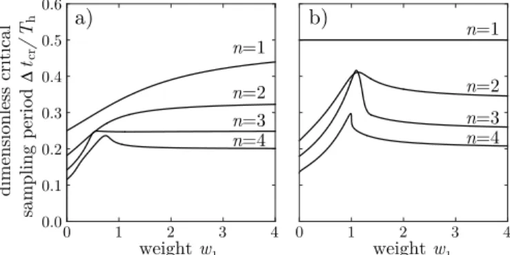
The size of the stable region depends on the sampling period as discussed in Section IV. Above a critical sampling period, t > tcr, the plant and string stable domain vanishes. For different packet loss scenarios, that is, for different values of n, the critical sampling period can be calculated by locating the intersection points of the string stability boundaries, and deter- mining the sampling period where they coincide; see details of the n=1 case in Appendix. The first row of Table I shows the critical sampling period for n =1,2,3,4, respectively. It is important to note that the more frequent the packet losses get,

(8)

the smaller the critical sampling period becomes. Hence frequent packet losses destabilize the system if the sampling time is not small enough. Note that the results in Table I also show that for a given t, the minimum achievable time gap Th=1/V(h^∗)between the vehicles increases as the packets are lost, that is, the maximum achievable flux in the traffic flow decreases.

In addition, it is important to note that large control gains imply large acceleration that the follower’s engine may not be able to realize or may not be permitted in the presence of human passengers. When the controller gets into saturation, the linear stability analysis is not valid any more. The minimum gains that make the system string stable are shown in Fig. 5 by enlarging the stable region around the origin.

The closest string stable points to the origin (whereα²+β²is minimal) are also indicated by red stars on the inlets. Notice that the smallest available gains increase when packets are lost.

VI. COMPENSATION OFPACKETLOSSES VIAPREDICTION

In this section, we propose a method to compensate for the destabilizing effects of the increasing time delay induced by packet losses. The method is based on the prediction of the leader’s velocity and the headway data lost during communication. Accordingly, we use a predicted headway h^P and a predicted leader’s velocity v^P_L in the control law:

˙

vF(t)=ades(tk−1), t ∈ [tk,tk+1), ades(tk−1)=α

V

h^P(tk−1)

−vF(tk−1) +β

W

v^PL(tk−1)

−vF(tk−1)

, (44) cf. (35).

To predict the leader’s velocity we use earlier data. More precisely, we propose to compute the predicted leader’s veloc- ity as a weighted sum (average) of the last m available leader’s velocity data:

v_L^P(tk−1)= m i=1

wivL(tk−τi(k)), (45) where the weights are indicated by wi and can be chosen when designing the predictor. The weights wi must satisfy _m

i=1wi = 1 in order to preserve the equilibrium velocity of the uniform flow for the nonlinear system (1), (44).

Parameter m denotes how many previously received data pack- ets are used for computing the predicted leader’s velocity – here we keep this fixed, independent of time. Parametersτi(k) indicate how many time steps earlier were the particular data packets received. For instance, if at tk the last two leader’s velocity data arrived 3 and 7 time steps ago, then τ1(k)=3 and τ2(k) = 7, and using both of these in the prediction corresponds to m=2. Note that the data packets may not be evenly distributed in time and any packet loss scenario can be described byτi(k). In the special case where every n-th packet is received and the last packet arrivedτ(k)time steps earlier, τi(k)=τ(k)+(i−1)n, i =1,2, . . . ,m.

By definition, the headway is the difference of the distances traveled by the leader and the follower. We can predict this

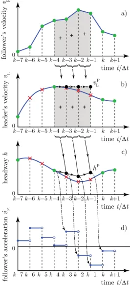
Fig. 6. Illustration of the prediction and the control processes with prediction algorithm (45)-(46) and control law (44) for m =1, w1 =1, τ1(k) = 4.

(a) (b) and (c) Green dots and red crosses show received and lost data packets, respectively, black dots show predicted data. Dashed arrows indicate the data used for leader’s velocity prediction, whereas the shaded areas and the solid arrows show the data used for headway prediction. (d) Dashed-dotted arrows show which data is used by the controller to set the follower’s acceleration.

by integrating (1). The key point is how we approximate the integrals of vL(t) and vF(t). Since the controller prescribes a piecewise constant acceleration for the follower, the velocity vF(t)is piecewise linear. Hence, we predict the distance that the follower travels by approximating the area undervF(t) by trapezoids; see Fig 6(a). Whereas we predict the distance that the leader travels by approximating the area undervL(t) by a rectangle using the predicted velocity v_L^P; see Fig 6(b).

The predicted headway becomes

h^P(tk−1)=h(tk−τ(k))+vL^P(tk−1)(τ(k)−1)t

−

τ(k)−1 j=1

vF(tk−j−1)+vF(tk−j)

2 t, (46)

for τ(k) ≥ 2. For τ(k) = 1, no packet is lost and we omit the sum in (46) to get h^P(tk−1) = h(tk−1). Thus no headway prediction is done when a packet is received. Note, however, that the leader’s velocity is predicted by (45) even

(9)

forτ(k)=1, so there is a possibility to improve string stability properties even when no packets are lost.

The method (45)-(46) to predict the leader’s velocity and the headway is illustrated in Fig. 6 for the special case m = 1, w1 = 1, τ1(k) = 4, that is, when the predictor relies on the data obtained 4 sampling periods earlier. Blue curves show the follower’s velocity, the leader’s velocity, the headway, and the follower’s acceleration as a function of time. Green dots indicate when packets are received and red crosses stand for packet losses. In case of packet losses, the leader’s velocity and the headway are predicted as shown by the black dots. The choice m =1 yields that the leader’s velocity is predicted to be the same as the last available data:

v^P_L(tk−1) = vL(tk−τ(k)), see the dashed arrows in Fig. 6(b).

This way, the controller assumes that the leader’s velocity does not change during packet losses, and the distance that the leader travels is computed accordingly. The headway is predicted by (46) by adding the difference of the distances that the leader and the follower travel during packet losses to the last available headway data; see the shaded areas and the solid arrows in Fig. 6(a,b,c). The dashed-dotted arrows in Fig. 6(d) show how the follower’s acceleration is set according to the control law (44).

Another special case of predictor (45)-(46) is when m=2, that is, the predictor uses the last two available leader’s velocity values obtainedτ1(k)andτ2(k)time instants earlier.

Then, the leader’s predicted velocity in Fig. 6(b) changes to v^P_L(tk−1) = w1 vL(tk−τ1(k))+w2 vL(tk−τ2(k)), where w2 = 1−w1. Ifw1=1 andw2=0, we get back the case m=1.

If w1 = w2 = 1/2, the leader’s velocity is predicted to be the average of the last two available leader’s velocity data, and the headway predictor (46) uses this average velocity to calculate the distance that the leader travels during packet losses. It is also possible to predict the leader’s velocity by linear extrapolation from the last two available data by choosingw1=(τ2(k)−1)/(τ2(k)−τ1(k))andw2=1−w1. Note that the choice of m and wi does not modify the prediction of the distance that the follower travels shown by the shaded area in Fig 6(a).

Now we solve (1), (44)-(46) with (12) along[tk,tk+1), and linearize the resulting discrete-time map, which yields X(k+1)=A^P_τ(_k₎X(k)+B0u(k)+B2u(k−2)

+ m

i=1

wiB^P_τ(_k₎u

k−τi(k) , (47)

where

A^P_τ(_k₎=A_τ(k)+A_τ(k), B^P_τ(_k₎=B_τ+B_τ(k), (48) and

A_τ(k)=

⎡

⎢⎢

⎢⎣

0 a^P/2 a^P · · · a^P a^P/2 0 · · · 0 0 I 0 · · · 0 0

0 I · · · 0 0

... ... ... ... ...

0 0 · · · I 0

⎤

⎥⎥

⎥⎦,

B_τ(k) =

⎡

⎢⎢

⎢⎣ b^P_τ(_k₎

o...

o

⎤

⎥⎥

⎥⎦, a^P =

0 1

2αV(h^∗)t³ 0 −αV(h^∗)t²

,

b^P_τ(_k₎ = −1

2(τ(k)−1)αV(h^∗)t³ (τ(k)−1)αV(h^∗)t²

, (49)

where there areτ(k)nonzero blocks in the first row ofA_τ(k), cf. (38), (39).

The stability analysis in the presence of the predictor can be done the same way as discussed in Section IV. The second and third rows of Fig. 5 show the stability diagrams using predictor (45)-(46) with m =1 and with m =2, w1=1/2, respectively, for n=1,2,3,4. The color and shading scheme is the same as used in Fig. 4(a). We can assess the effect of predictor (45)-(46) by comparing the rows of Fig. 5.

Based on the first row of Fig. 5, the plant stable domains vary significantly for the different packet loss scenarios when no predictor is used. In comparison, the second and third rows of Fig. 5 show that these domains remain exactly the same using predictor (45)-(46) as for no packet loss and no prediction, cf. Fig. 5(a). This implies that plant stability can be preserved by implementing predictors on the headway. The reason of the robustness of plant stability with respect to packet losses is the following. During plant stability analysis, we investigate stability in the absence of the leader’s velocity fluctuations. Thus, only the headway needs to be predicted in order to improve plant stability. Since the follower’s velocity is not affected by packet losses, it is available for the controller and can be integrated to obtain the exact headway for any packet loss scenario. This leads to the preservation of plant stability properties.

According to the first and second rows of Fig. 5, the choice m = 1 fails to increase the size of the string stable region.

However, by choosing m =2, the weightw1 can be used as a design tool for enhancing string stability properties. Based on several case studies, the optimal choice of w1 in terms of the size of the string stable region is around w1 = 1/2;

see the third row of Fig. 5. A heuristic argument supporting this choice is the following. When every n-th packet is delivered, the relation between v^P_L(tk−1)and vL(tk−τ(k)) can be characterized by the transfer function^P(z)=w1+w2z⁻ⁿ wherew2=1−w1. Consequently, prediction introduces a gain and a phase shift in the leader’s velocity. The square of the gain is obtained as^P

eⁱ^ω^t²=1−4w1(1−w1)sin²(nωt/2), which is minimal forw1=1/2. Indeed, we see improvements of string stability when applying the predictor with m = 2, w1=1/2 in the third row of Fig. 5. The string stable regions become larger compared to the first row of Fig. 5, especially for frequent packet losses (n=3,4).

It is important to highlight that for m = 2, the weight w1=1/2 is optimal in terms of the size of the stable region.

This choice may not be optimal in terms of the minimal gains that make the system string stable. According to the second and third rows of Fig. 5, smaller gains can be achieved for w1 = 1 (which gives case m = 1) than for w1=1/2 as highlighted by the inlets. We can also analyze the effect of