37(2010) pp. 165–175
http://ami.ektf.hu
Geometric properties and constrained modification of trigonometric
spline curves of Han
Ede M. Troll, Miklós Hoffmann
∗Institute of Mathematics and Computer Science Eszterházy Károly College
Submitted 25 March 2010; Accepted 10 August 2010
Dedicated to professor Béla Pelle on his 80th birthday
Abstract
New types of quadratic and cubic trigonometrial polynomial curves have been introduced in [2] and [3]. These trigonometric curves have a global shape parameterλ. In this paper the geometric effect of this shape parameter on the curves is discussed. We prove that this effect is linear. Moreover we show that the quadratic curve can interpolate the control points atλ=√
2. Constrained modification of these curves is also studied. A curve passing through a given point is computed by an algorithm which includes numerical computations.
These issues are generalized for surfaces with two shape parameters. We show that a point of the surface can move along a hyperbolic paraboloid.
Keywords:trigonometric curve, spline curve, constrained modification MSC:68U07, 65D17
1. Introduction
In Computer Aided Geometric Design the most prevalently used curves are B- Spline and NURBS curves. Besides the quadratic and the cubic B-Spline and NURBS curves the trigonometric spline curves are another way to define curves above a new function space. Among the first ones, C-Bézier and uniform CB-spline
∗The second author was supported by the János Bolyai Fellowship of the Hungarian Academy of Science.
165
curves are defined by means of the basis{sint,cost, t,1}, which was generalized to {sint,cost, tk−3, tk−4, . . . , t,1}(cf. [14, 15, 16, 1]). Wang et al. introduced NUAT B-spline curves ([13]) that are the non-uniform generalizations of CB-spline curves.
The other basic type is the HB-spline curve, the basis of which is{sinht,cosht, t,1}, and {sinht,cosht, tk−3, tk−4, . . . , t,1} in higher order ([12, 9]). Li and Wang de- veloped its non-uniform generalization ([8]). Trigonometric curves can produce several kinds of classical important curves explicitly due to their trigonometric basis functions, including circle and circular cylinder [14], ellipse [16], surfaces of revolution [11], cycloid [10], helix [12], hyperbola and catenary [9]. Two recently defined trigonometric curves are the quadratic [2] and cubic [3] trigonometric curves of Xuli Han. The aim of this paper is to discuss the geometric properties of these curves, including the effect of their shape parameters and the possibility of con- strained modification of the curves by these parameters. The method of our study is similar to the papers discussing geometric properties and modification of other types of spline curves. Such research has been done e.g. for C-Bézier curves [6], FB-spline curves [4], GB-spline curves [7] and another quartic curve of Han [5].
In this paper the definition of quadratic and cubic trigonometric polynomial curves are presented in Section 2. The geometric effects of the shape parameter as well as its application for constrained modification are discussed for quadratic curve in Section 3. These results are extended for the cubic case in Section 4, and for quadratic trigonometric surfaces in Section 5.
2. Definition of the basis functions
The construction of the basis functions of the quadratic trigonometric curve is the following [2].
Definition 2.1. Given knotsu0< u1<· · ·< un+3, let
∆ui:=ui+1−ui, ti(u) :=π 2
u−ui
∆ui
, αi:= ∆ui
∆ui−1+ ∆ui
, c(t) := 1−sin(t)
1−λsin(t) , βi:= ∆ui
∆ui−∆ui+1, d(t) := 1−cos(t)
1−λcos(t) ,
where −1< λ <1. Then the associated trigonometric polynomial basis functions are defined to be the following functions:
bi(u) =
βid(ti), u∈[ui, ui+1), 1−αi+1c(ti+1) +βi+1d(ti+1), u∈[ui+1, ui+2), αi+2c(ti+2), u∈[ui+2, ui+3),
0, u /∈[ui, ui+3),
fori= 0,1, . . . , n.
In [2] the author proves several theorems in terms of this new curve, but the most important ones are the following: ifλ= 0, then the trigonometric polynomial curve is an arc of an ellipse and the basis functionbi(u)hasC1 continuity at each of the knots.
The definition of the cubic trigonometric polynomial curve in [3] is as follows.
Definition 2.2. Given knotsu0< u1<· · ·< un+4 and refer toU = (u0, u1, . . . , un+4)as a knot vector. Forλ∈Rand all possiblei∈Z+, let∆i=ui+1−ui,
αi= ∆i−∆1+∆i i, βi= ∆i+∆∆ii+1, γi= ∆i−1+(2λ+1)∆1 i+∆i+1, ai= ∆iαiγi−1, di= ∆iβiγi+1,
bi2= 4λ+61 (∆i+1−∆i)γi, ci1= 4λ+61 (∆i−1−∆i)γi, bi0= ∆i−1αiγi−ai+bi2, ci0= [1−(2λ+ 3)αi]ci1, bi1= 12∆iγi+bi2, ci2= 12∆iγi+ci1, bi3= [1−(2λ+ 3)βi]bi2, ci3= ∆i+1βiγi+ci1−di,
f0(t) = (1−sin(t))2(1−λsin(t)), f1(t) = (1 + cos(t))2(1 +λcos(t)), f2(t) = (1 + sin(t))2(1 +λsin(t)), f3(t) = (1−cos(t))2(1−λcos(t)).
Given a knot vector U, let tj(u) = π2u−∆ujj (j = 0,1, . . . , n+ 3), the associated trigonometric polynomial basis functions are defined to be the following functions:
Bi(u) =
dif3(ti), u∈[ui, ui+1), P3
j=0ci+1,jfj(ti+1), u∈[ui+1, ui+2), P3
j=0bi+2,jfj(ti+2), u∈[ui+2, ui+3), ai+3f0(ti+3), u∈[ui+3, ui+4), 0, u /∈[ui, ui+4), fori= 0,1, . . . , n.
3. The quadratic case
3.1. Geometric effect of the shape parameter
The basis functions of the quadratic trigonometric polynomial curve have a shape parameter λ∈ (−1,1), (see Section 1). For our works we restrict the domain of definition of the basis functions to one span. Let u∈[ui, ui+1), then
bi(u) =
ui+1−ui
ui+2+ui
1−cos π
2
u−ui
ui+1−ui
!
1−λcos π
2
u−ui
ui+1−ui
! ,
bi−1(u) = 1−
ui+1−ui
ui−1+ui+1
1−sin π
2
u−ui
ui+1−ui
!
1−λsin π
2
u−ui
ui+1−ui
!
−
ui+1−ui
ui+2+ui
1−cos π
2
u−ui
ui+1−ui
!
1−λcos π
2 u−ui
ui+1−ui
! ,
bi−2(u) =
ui+1−ui
ui−1+ui+1
1−sin π
2
u−ui
ui+1−ui
!
1−λsin π
2
u−ui
ui+1−ui
! , hence one arc of the quadratic trigonometric polynomial curve is
Ti(u, λ) =bi−2(u)pi−2+bi−1(u)pi−1+bi(u)pi, wherepi are the control points.
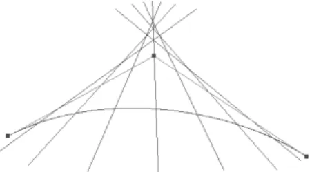
Theorem 3.1. The geometric effect of the shape parameter is linear, that is if u0∈[ui, ui+1)is fixed, then the curve pointTi(u0, λ)moves along a line segment.
Proof. Parts of basis functions not containing the shape parameterλcan be con- sidered as constants:
k1=u
i+1−ui ui+2+ui
1−cos
π 2
u0−ui ui−1−ui
, k2= cos
π 2
u0−ui ui−1−ui
, k3= u
i+1−ui ui+1+ui−1
1−sin
π 2
u0−ui ui−1−ui
, k4= sin
π 2
u0−ui ui−1−ui
.
By these constants the basis functions of the quadratic trigonometric polynomial curve can be expressed as:
bi−2(u0, λ) =k3−λk3k4,
bi−1(u0, λ) = 1−k3+λk3k4−k1+λk1k2, bi(u0, λ) =k1−λk1k2.
Thus the path of the curve point at parameteru0is T(u0, λ) = (k3−λk3k4)pi
−2+ (1−k3+λk3k4−k1+λk1k2)pi
−1+ (k1−λk1k2)pi, which yields an equation of a line segment
T(u0, λ) = k3pi
−2+ (1−k1−k3)pi−2+k1pi +λ k3k4(pi−1−pi
−2) +k1k2(pi−1−pi) .
The theorem follows.
3.2. Common interpolation
Interpolation of points in general is possible by any of the spline curves by a reverse algorithm: considering the pointsp0,p1, . . . ,pnto be interpolated by the curve, the new control points can be computed. This algorithm, however, generally requires time-consuming computation solving a system of equations. Thus it can be useful to study if the curve (if it includes a shape parameter) can directly interpolate the given points at a proportional value of the shape parameter.
Figure 1: The geometric effect of the shape parameter with fixed parameter u0. Straight lines show the λ-paths of the quadratic
trigonometric curve.
Theorem 3.2. The quadratic trigonometric polynomial curve interpolates the con- trol points atλ=√
2.
Proof. Let the control points p0,p1,p2 soui−1= 0, ui = 0, ui+1 = 1, ui+2 = 1 and the parameter where we search the interpolation is u= ui+u2i+1 hence
bi(u) = 1−cos π
4 !
1−√ 2cos
π 4
!
= 0,
bi−1(u) = 1− 1−cos π
4 !
1−√ 2cos
π 4
!
− 1−sin π
4 !
1−√ 2sin
π 4
!
= 1,
bi−2(u) = 1−sin π
4 !
1−√ 2sin
π 4
!
= 0.
The theorem follows.
Figure 2: The quadratic trigonometric polynomial curve withλ=
√2interpolates the control points, having end tangents parallel to the sides of the control polygon.
3.3. Constrained modification
In Computer Aided Geometric Design a frequent problem is the constrained modifi- cation, when control points are given and we have another pointpwhat we need to interpolate by the curve, possibly by altering the parameters of the curve. Our aim is to modify the given curveT(u, λ)by altering exclusively the shape parameter in a way, that the modified curve will pass through the given point, that is, for some parameters T(¯u,λ) =¯ p. The first observation to create this interpolation with the quadratic trigonometric polynomial curve is to show how we could produce a segment with this curve.
Lemma 3.3. Let the control points bepi
−2,pi
−1,pi. Ifλ=−1, then the quadratic trigonometric curve is a line segment between pi
−2 andpi. Proof. Let the curve segment be
Ti(u0,−1) =pi
−1+A(pi−2−pi
−1) +B(pi−pi
−1), whereA=k3−λk3k4,B=k1−λk1k2, andA+B= 1, therefore
Ti(u0,−1) =Api
−2+ (1−A)pi.
The theorem follows.
Figure 3: Constrained modification on the quadtaric trigonometric polynomial curve.
For a fixed parameter u0 one can also find the intersection of the λ-path as- sociated to u0 and the control polygon. In the first case, when0 6u0 60,5 we can find the parameter value λ0 at which B = 0. Since B = k1−λk1k2 = 0, thereforeλ0= k1
2. So the intersection point isT(u0,k1
2). In the second case, when 0,5 < u061 thenA= 0 should hold. A=k3−λk3k4 yieldsλ0 = k1
4. Thus the point what we are looking for isT(u0,k1
4). Since lambda paths are line segments, they can be described by the two pointsTi(u0,−1)andTi(u0, λ0). Our next task
is to find the valueu¯for which the pathT(¯u, λ)passes troughp, by elementary in- cidence computation. Finally the value of¯λcan be found by a numerical algorithm for which
T(¯u,¯λ) =p.
holds. From the algorithm it is clear that the admissible positions of p can be inside the convex hull of the control points.
4. Extension to the cubic case
The cubic trigonometric polynomial curve also has a shape parameter λ∈R(see Section 1), and we need the following remark from [3].
Remark 4.1. Ifui6=ui+1(36i6n), then foru∈[ui, ui+1], the curveT(u)can be represented by curve segment
T(u) =Bi−3pi
−3+Bi−2pi
−2+Bi−1pi
−1+Bipi. With a uniform knot vector, we have
Bi−3(u) = 4λ+6f0(t), Bi−2(u) =4λ+6f1(t), Bi−1(u) = 4λ+6f2(t), Bi(u) = 4λ+6f3(t), wheret=π(u−ui)/(2∆i).
Theorem 4.2. With a uniform knot vector ifu0∈[ui, ui+1)is fixed, then the ge- ometric effect of the shape parameter is linear, i.e. theλ-path of the pointT(u0, λ) of the curve are straight line segments.
Proof. The derivatives of the basis functions with respect to λare δBi−3
δλ =
−(1−sin(t))2sin(t)
(4λ+ 6)−4(1−sin(t))2(1−λsin(t))
(4λ+ 6)2 =
=−(−1 + sin(t))2(2 + 3 sin(t)) 2(3 + 2λ)2 , δBi−2
δλ =
(1 + cos(t))2cos(t)
(4λ+ 6)−4(1 + cos(t))2(1 +λcos(t))
(4λ+ 6)2 =
= (1 + cos(t))2(−2 + 3 cos(t)) 2(3 + 2λ)2 , δBi−1
δλ =
(1 + sin(t))2sin(t)
(4λ+ 6)−4(1 + sin(t))2(1 +λsin(t))
(4λ+ 6)2 =
= (1 + sin(t))2(−2 + 3 sin(t)) 2(3 + 2λ)2 , δBi
δλ =
−(1−cos(t))2cos(t)
(4λ+ 6)−4(1−cos(t))2(1−λcos(t))
(4λ+ 6)2 =
=−(−1 + cos(t))2(2 + 3 cos(t)) 2(3 + 2λ)2 ,
hence the derivative of the cubic trigonometric polynomial curve with respect toλ is
δT
δλ = 1
2(3 + 2λ)2 (−1 +sin(t))2(2 + 3sin(t))p0
+ (1 + cos(t))2(−2 + 3 cos(t))p1+ (1 + sin(t))2(−2 + 3 sin(t))p2 + (−1 + cos(t))2(2 + 3 cos(t))p3
.
In the domain ofT(u0, λ)all the derivative vectors of theλ-paths with respect to λ point to the same direction, λ alters only the derivatives lengths. This proves
the statement.
Figure 4: The geometric effect of the shape parameter is linear in the cubic case as well,λ-paths are line segments.
Sinceλ-paths belong to a fixedu0 are line segments in the cubic case as well, constrained modification can be computed analogously to the quadratic case (cf.
Fig. 5).
Figure 5: Constrained modification on the cubic trigonometric polynomial curve.
5. Extension to surfaces
In this section we present the quadratic trigonometric polynomial surface which is a tensor product surface obtained by the quadratic curve. The basis functions are as follows
bi(u) =
ui+1−ui
ui+2+ui
1−cos π
2
u−ui
ui+1−ui
!
1−λucos π
2
u−ui
ui+1−ui
! ,
bi−1(u) = 1−
ui+1−ui
ui−1+ui+1
1−sin π
2
u−ui
ui+1−ui
!
1−λusin π
2
u−ui
ui+1−ui
!
−
ui+1−ui
ui+2+ui
1−cos π
2
u−ui
ui+1−ui
!
1−λucos π
2
u−ui
ui+1−ui
! ,
bi−2(u) =
ui+1−ui
ui−1+ui+1
1−sin π
2
u−ui
ui+1−ui
!
1−λusin π
2
u−ui
ui+1−ui
! ,
bi(v) =
vi+1−vi
vi+2+vi
1−cos π
2
v−vi
vi+1−vi
!
1−λvcos π
2
v−vi
vi+1−vi
! ,
bi−1(v) = 1−
vi+1−vi
vi−1+vi+1
1−sin π
2
v−vi
vi+1−vi
!
1−λvsin π
2
v−vi
vi+1−vi
!
−
vi+1−vi
vi+2+vi
1−cos π
2
v−vi
vi+1−vi
!
1−λvcos π
2
v−vi
vi+1−vi
! ,
bi−2(v) =
vi+1−vi
vi−1+vi+1
1−sin π
2
v−vi
vi+1−vi
!
1−λvsin π
2
v−vi
vi+1−vi
! , where−1< λu, λv <1 are shape parameters, and the surface patch is defined as
T(u, v) =bi−2(u)bi−2(v)pj+bi−2(u)bi−1(v)pj+1+bi−2(u)bi(v)pj+2+ +bi−1(u)bi−2(v)pj+3+bi−1(u)bi−1(v)pj+4+bi−1(u)bi(v)pj+5+ +bi(u)bi−2(v)pj+6+bi(u)bi−1(v)pj+7+bi(u)bi(v)pj+8.
The shape parameters λu, λv are independent so they modify the surface in sep- arated ways. As we have seen for λ= −1 the quadratic curve is a line segment passing through pi
−2 and pi. Consequently the quadratic trigonometric polyno- mial surface at λu = −1 and λv = −1 is a plane interpolating control points pj,pj+2,pj+6,pj+8.
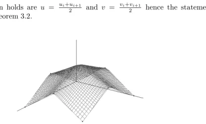
Theorem 5.1. The quadratic trigonometric polynomial surface interpolates the control points when λu=√
2 andλv =√ 2.
Proof. Considering the control pointspk (k= 1,2, . . . ,9), knotsui−1= 0,ui= 0, ui+1= 1,ui+2= 1,vi−1= 0,vi = 0,vi+1 = 1, vi+2= 1, the parameters at which
the interpolation holds are u = ui+u2i+1 and v = vi+v2i+1 hence the statement
follows from Theorem 3.2.
Figure 6: The quadratic trigonometric polynomial surface with λu=√
2andλv=√ 2.
5.1. Geometric effect of the shape parameters λ
uand λ
von the quadratic trigonometric surface
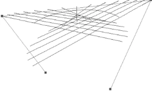
Since shape parameters acts independently on the surface, if we fix either of them, the geometric effect of the other shape parameter is the same as in the curve case (see Section 3.1). Consequently in the case when both of the shape parameters are changing simultaneously, points of the surface can move on a doubly ruled surface, an example of which can be seen in Fig.7.
Figure 7: λ-paths of a surface point associated tou0 = 0,2 and v0 = 0,2are on a hyperbolic paraboloid (one of its section curves
is also shown).
References
[1] Chen, Q., Wang, G., A class of Bézier-like curves, Computer Aided Geometric Design, 20, (2003) 29–39.
[2] Han, X., Quadratic trigonometric polynomial curves with a shape parameter,Com- puter Aided Geometric Design, 19 (2002) 503–512.
[3] Han, X., Cubic trigonometric polynomial curves with a shape parameter,Computer Aided Geometric Design, 21 (2004) 535–548.
[4] Hoffmann, M., Juhász, I., Modifying the shape of FB-spline curves, Journal of Applied Mathematics and Computing, 27, (2008) 257–269.
[5] Hoffmann, M., Juhász, I., On the quartic curve of Han,Journal of Computational and Applied Mathematics, 223, (2009) 124–132.
[6] Hoffmann, M., Li, Y., Wang, G., Paths of C-Bézier and C-B-spline curves, Computer Aided Geometric Design, 23, (2006) 463–475.
[7] Li, Y., Hoffmann, M., Wang, G., On the shape parameter and constrained modification of GB-spline curves,Annales Mathematicae et Informaticae, 34, (2007) 51–59.
[8] Li, Y., Wang, G., Two kinds of B-basis of the algebraic hyperbolic space,Journal of Zheijang Univ. Sci., 6, (2005) 750–759.
[9] Lü, Y., Wang, G., Yang, X., Uniform hyperbolic polynomial B-spline curves, Computer Aided Geometric Design, 19, (2002) 379–393.
[10] Mainar, M., Pena, J.M., Sanchez-Reyes, J., Shape preserving alternatives to the rational Bézier model.Computer Aided Geometric Design, 18, (2001) 37–60.
[11] Morin, G., Warren, J., Weimer, H., A subdivision scheme for surface of revo- lution,Computer Aided Geometric Design, 18, (2001) 483–502.
[12] Pottmann, H., The geometry of Tchebycheffian splines,Computer Aided Geometric Design, 10, (1993) 181–210.
[13] Wang, G., Chen, Q., Zhou, M., NUAT B-spline curves,Computer Aided Geo- metric Design, 21, (2004) 193–205.
[14] Zhang, J.W., C-curves, an extension of cubic curves, Computer Aided Geometric Design, 13, (1996) 199–217.
[15] Zhang, J.W., Two different forms of CB-splines,Computer Aided Geometric Design, 14, (1997) 31–41.
[16] Zhang, J.W., C-Bézier curves and surfaces, Graph. Models Image Process., 61, (1999) 2–15.
Ede M. Troll, Miklós Hoffmann
Institute of Mathematics and Computer Science Eszterházy Károly College
Leányka str. 4 Eger
Hungary
e-mail: ede.troll@gmail.com hofi@ektf.hu