Constrained modification of the cubic trigonometric Bézier curve with two shape
parameters
Ede Troll
University of Debrecen ede.troll@gmail.com
Submitted September 13, 2014 — Accepted December 7, 2014
Abstract
A new type of cubic trigonometric Bézier curve has been introduced in [1]. This trigonometric curve has two global shape parametersλandµ. We give a lower boundary to the shape parameters where the curve has lost the variation diminishing property. In this paper the relationship of the two shape parameters and their geometric effect on the curve is discussed. These shape parameters are independent and we prove that their geometric effect on the curve is linear. Because of the independence constrained modification is not unequivocal and it raises a number of problems which are also studied. These issues are generalized for surfaces with four shape parameters. We show that the geometric effect of the shape parameters on the surface is parabolic.
Keywords:trigonometric curve, spline curve, constrained modification MSC:AMS classification numbers
1. Introduction
Although classical polynomial curves, such as Bézier curve and B-spline curve still play central role in computer aided geometric design, several new curves have been developed in the last decade. The basic principle of curve design is still valid: the curve is given by user-defined points (so-called control points) which are combined with predefined basis functions. Keeping this principle in mind, the generalizations show various directions of possible improvements in theory and practice as well,
http://ami.ektf.hu
145
applying basis functions different from the polynomial ones. In several cases the reason for this is either to provide a curve description method which can exactly describe (and not only approximate) important classical curves, which cannot be done by polynomial basis functions, or to simplify the computation of the curves and their properties. The most well-known generalization is the rational Bézier and B-spline curve [5], where rational functions are applied as basis functions, but deriving these functions one can obtain high degree rational polynomials, which may cause stability problems computing higher order derivatives.
The other way to improve the abilities of such a curve is the application of trigonometric functions. Trigonometric spline curves can also represent important curves, such as circle, lemniscate, etc. exactly, which cannot be done by polynomial curves. The theoretical fundamentals for this kind of curves have been laid in [10]. C-Bézier and uniform CB-spline curves are defined by means of the basis {sint,cost, t,1}, that was generalized to {sint,cost, tk−3, tk−4, . . . , t,1} [11, 12, 13]. NUAT B-spline curves introduced by Wang et al. in [15], the non-uniform generalizations of CB-spline curves. The other basic type is the HB-spline curve, the basis of which is {sinht,cosht, t,1}, and {sinht,cosht, tk−3, tk−4, . . . , t,1} in higher order [14, 10].
Another, not necessarily independent direction of generalization is the incor- poration of shape parameters to the basis functions in order to provide additional freedom in shape adjustment. One of the earliest methods in this way is β-spline curve with two global parameters [7, 8]. Further methods have been provided by direct generalization of B-spline curves asαB-splines in [9] and [6] and recently as GB-splines in [4]. A spline curve with exponential shape parameters is defined and studied in [28]. Some alternative spline curves with shape parameters can be found in [2, 3, 29]. HB-spline curves, CB-spline curves and the uniform B-spline curves have been unified under the name of FB-spline curves in [16, 17]. The evaluation of these trigonometric spline curves are more stable than that of NURBS curves [18, 19].
In the above mentioned papers the new curve types are defined and essential properties are proved, but the more detailed geometric analysis of the curve has not been provided, however, it is of great importance in applications. ‘How the shape parameters influence the shape of the curve?’ and ‘How the curve can be applied for interpolation problems?’ are just two of these questions. Constrained modification of the curves is also a central issue of applications. These questions are studied in several papers [20, 23, 24, 28, 26, 27].
The aim of this paper is to study the geometrical properties of a recently defined new curve type. Our methods for finding paths of the curve points (Section 3) and describing constrained modification (Section 4) follow the techniques developed in [21] and [22] for B-spline and NURBS curves.
In [1] the authors defined a new type of curves called T-Bézier curve as follows.
Definition 1.1. For two arbitrarily selected real values of λandµ, whereλ, µ ∈ [−2,1], the following four functions oft(t∈[0,1])are defined as cubic trigonometric
Bézier (i.e. T-Bézier) basis functions with two shape parameters λandµ:
b0(t) =
1−sinπt 2
2
1−λsinπt 2
b1(t) = sinπ
2
1−sinπ 2
2 +λ−λsinπt 2
b2(t) = cosπ
2
1−cosπ 2
2 +µ−µcosπt 2
b3(t) =
1−cosπt 2
2
1−µcosπt 2
In the following sections we study the variation diminishing property, the effect of the shape parameters for the curve and the constrained modification abilities of this curve. Finally, the curve type is generalized for surfaces.
2. Variation diminishing
In the following, we will discuss new properties of the T-Bézier curve. In CAD systems the variation diminishing property is necessary for a Bézier curve. When we define a control polygon for a curve then we expect that the number of intersections with the produced curve will be less than or equal to the number of intersections with the defined control polygon.
Theorem 2.1. Ifλ <−2orµ <−2than the T-Bézier curve has lost its variatonal diminishing property.
Proof. The derivatives of the basis functions with respect to a variable tare δb0
δt =1 2cosπt
2 3 cosπt 2
2
λ+ 4λsinπt
2 + 2 sinπt
2 −4λ−2
! π, δb1
δt =−1 2cosπt
2 3 cosπt 2
2
λ+ 4λsinπt
2 + 4 sinπt
2 −4λ−2
! π, δb2
δt =−1 2sinπt
2 3 cosπt 2
2
µ−4µcosπt
2 −4 cosπt
2 +µ+ 2
! π, δb3
δt =1 2sinπt
2 3 cosπt 2
2
µ−2µcosπt
2 −4 cosπt
2 +µ+ 2
! π, and
δb0
δt(0) =−1
2πλ−π, δb0
δt (1) = 0, δb1
δt(0) = 1
2πλ+π, δb1
δt (1) = 0,
δb2
δt(0) = 0, δb2
δt (1) =−1
2πµ−π, δb3
δt(0) = 0, δb3
δt (1) =1
2πµ+π.
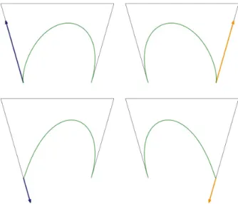
With the control points p0,p1,p2,p3 the tangent vectors at the points at t = 0 andt= 1areπ 12λ+ 1
(p1−p0)andπ 12µ+ 1
(p3−p2)respectively, therefore if λ <−2, than the direction of the tangent vector at the point att= 0is opposite to the vector(p1−p0), and ifµ <−2, then the direction of the tangent vector at the point att= 1is opposite to the vector(p3−p2). The theorem follows.
Figure 1: The tangent vectors at points att= 0with λ=−1,5 on the top left,t= 0withλ=−2,2on the bottom left,t= 1with µ=−1,5on the top right andt= 1withµ=−2,2on the bottom
right
3. The geometric effect of the shape parameters
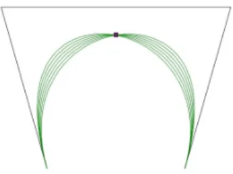
The basis functions of the cubic trigonometric Bézier curve are contain two arbi- trarily selected real values λandµ as shape parameters. When these parameters are changing the shape of the curve is altered too. If we have a given knot vector t0 and one of the shape parameters is fix, than we can examine the path of the T(t, λ, µ)point of the curve while the other shape parameter is varies between its boundaries.
Theorem 3.1. If t∈[0,1]andµ∈[−2,1]is a constant, then the geometric effect of the shape parameter λis linear.
Proof. Those basis function segments which does not include the shape parameter λ, we can expect as constants. Let
c0λ,t = sinπ 2t, c1λ,t = 1−sinπ
2t, c2λ,t = cosπ
2
1−cosπ 2
2 +µ−µcosπ 2t
, c3λ,t =
1−cosπ 2t2
1−µcosπ 2t
.
With these constants we can express the basis functions of the quadratic trigono- metric polynomial curve:
b0(t) =c21λ,t(1−λc0λ,t) =c21λ,t−λc0λ,tc21λ,t
b1(t) =c0λ,tc1λ,t(2 +λ−λc0λ,t) = 2c0λ,tc1λ,t+λc0λ,tc1λ,t−λc20λ,tc1λ,t
b2(t) =c2λ,t
b3(t) =c3λ,t
The theorem follows.
Figure 2: The geometric effect of the shape parameterλ
Theorem 3.2. If t∈[0,1]andλ∈[−2,1]is a constant, then the geometric effect of the shape parameter µis linear.
Proof. Those basis function segments which does not include the shape parameter µ, we can expect as constants. Let
c0µ,t = cosπ 2t, c1µ,t = 1−cosπ
2t, c2µ,t = sinπ
2
1−sinπ 2
2 +λ−λsinπ 2t
, c3µ,t =
1−sinπ 2t2
1−λsinπ 2t
.
With these constants we can express the basis functions of the quadratic trigono- metric polynomial curve:
b0(t) =c3µ,t
b1(t) =c2µ,t
b2(t) =c0µ,tc1µ,t(2 +µ−µc0µ,t) = 2c0µ,tc1µ,t+µc0µ,tc1µ,t−µc20µ,tc1µ,t
b3(t) =c21µ,t(1−µc0µ,t) =c21µ,t−µc0µ,tc21µ,t The theorem follows.
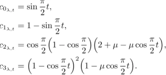
Figure 3: The geometric effect of the shape parameterµ
The two shape parameters are independent of each other so they modify the shape of the curve in separated ways. In a specific case we can examine the effect of the two parameters when they simultaneously changing their value.
Theorem 3.3. Ift∈[0,1]is a constant and we run both of the shape parameters at the same time, then the geometric effect of the shape parameters is linear.
Proof. Letk∈R,λ, µ∈[−2,1]andµ=kλ, and consider the constants c1λ,t, c2λ,t
from Theorem 3.1. With these constants we can express the basis functions of the quadratic trigonometric polynomial curve:
b0(t) =c22λ,t(1−λc1λ,t) =c22λ,t−λc1λ,tc22λ,t
b1(t) =c1λ,tc2λ,t(2 +λ−λc1λ,t) = 2c1λ,tc2λ,t+λc1λ,tc2λ,t−λc21λ,tc2λ,t
b2(t) =c1λ,tc2λ,t(2 +kλ−kλc1λ,t) = 2c1λ,tc2λ,t+kλc1λ,tc2λ,t−kλc21λ,tc2λ,t
b3(t) =c22λ,t(1−kλc1λ,t) =c22λ,t−kλc1λ,tc22λ,t The theorem follows.
Figure 4: The shape parameters’ geometric effect
4. Constrained modification
If a point p is given, than we need to find the values of the shape parameters λ, µ∈[−2,1]with which the curve interpolates the point. Let the curve be
T(t, λ, µ) = X3
i=0
bi(t)pi,
wherepi, i∈0,1,2,3 are the control points.
From the inordinate case when µ is fixed and only the value of λis changing to that case when λ is fixed everyλ =kµ, k ∈ R paths are intersects the curve.
Within the boundaries the curve can interpolate the pointpand the appropriate value of the running parameter depends on the values of the shape parameters.
Figure 5: The appropriate section of the curve for interpolation
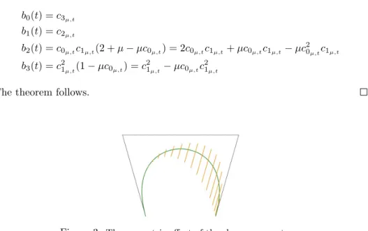
On the other hand, when we fix a point on the curve, then we can examine the paths we discussed above. In this case we can show the permissible area of the point of the curve.
Figure 6: The permissible area of a point of the curve
If we consider the union of the permissible areas for every point of the curve, than we get the permissible area of the whole curve.
Figure 7: The admissible area of the curve
As regards the above the constrained modification is unequivocal only when λ=µ. In this case with a numerical method we can produce the appropriate value of the running parametert0, whereby the produced line interpolate the given point p. Finally, the value of the shape parameters are given from
T(t0, λ, µ) =p, whereλ=µ.
Figure 8: Constrained modification of the curve
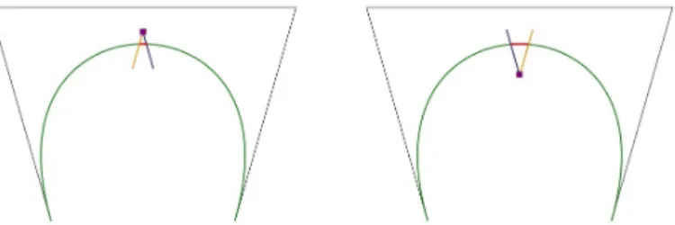
While we discussed the algorithm of the constrained modification, we have assumed that the shape parameters are equivalent λ = µ. This condition isn’t necessary, but if λ6=µ, the count of the cases when the curve can interpolate a given pointpis infinite.
Figure 9: Constrained modification of the curve with different shape parameter values
5. Extension to surfaces
The cubic trigonometric Bézier surface made from the basis functions of the T- Bézier curve. The shape parameters also modify the face of the surface with their value, like in the case of the curve. In three dimension we expect only the case when one of the two shape parameter is fix. In the other case (when we change the other shape parameters) the proof is the same.
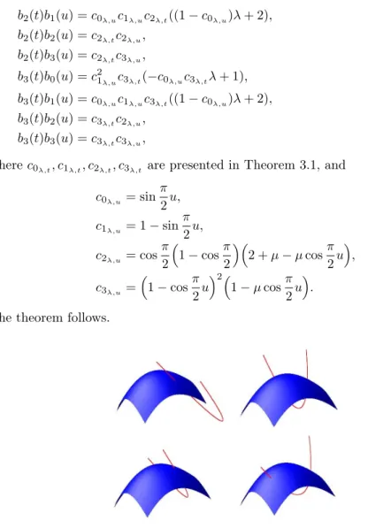
Theorem 5.1. If t, u ∈ [0,1] and µ ∈ [−2,1] is a constant, then the geometric effect of the shape parameter λis parabolic.
Proof. The cubic trigonometric Bézier surface is
T(t, u) = X3
i,j=0
bi(t)bj(u)pi,j, where
pi,j, i, j∈0,1,2,3
are the control points. Now we can express the coefficients.
b0(t)b0(u) =c21λ,tc21λ,u(c0λ,tc0λ,uλ2−(c0λ,t+c0λ,u)λ+ 1),
b0(t)b1(u) =c0λ,uc21λ,tc1λ,u(c0λ,t(c0λ,u−1)λ2−(2c0λ,t+c0λ,u−1)λ+ 2), b0(t)b2(u) =c21λ,tc2λ,u(−c0λ,tλ+ 1),
b0(t)b3(u) =c21λ,tc3λ,u(−c0λ,tλ+ 1),
b1(t)b0(u) =c0λ,tc1λ,tc21λ,u(c0λ,u(c0λ,t−1)λ2−(c0λ,t+ 2c0λ,u−1)λ+ 2), b1(t)b1(u) =c0λ,tc0λ,uc1λ,tc1λ,u((c0λ,t(c0λ,u−1)−c0λ,u+ 1)λ2
−(2c0λ,t+ 2c0λ,u−4)λ+ 4), b1(t)b2(u) =c0λ,tc1λ,tc2λ,u((1−c0λ,t)λ+ 2), b1(t)b3(u) =c0λ,tc1λ,tc3λ,u((1−c0λ,t)λ+ 2), b2(t)b0(u) =c21λ,uc2λ,t(−c0λ,uc2λ,tλ+ 1),
b2(t)b1(u) =c0λ,uc1λ,uc2λ,t((1−c0λ,u)λ+ 2), b2(t)b2(u) =c2λ,tc2λ,u,
b2(t)b3(u) =c2λ,tc3λ,u,
b3(t)b0(u) =c21λ,uc3λ,t(−c0λ,uc3λ,tλ+ 1), b3(t)b1(u) =c0λ,uc1λ,uc3λ,t((1−c0λ,u)λ+ 2), b3(t)b2(u) =c3λ,tc2λ,u,
b3(t)b3(u) =c3λ,tc3λ,u,
wherec0λ,t, c1λ,t, c2λ,t, c3λ,t are presented in Theorem 3.1, and c0λ,u= sinπ
2u, c1λ,u= 1−sinπ
2u, c2λ,u= cosπ
2
1−cosπ 2
2 +µ−µcosπ 2u
, c3λ,u=
1−cosπ 2u2
1−µcosπ 2u
. The theorem follows.
Figure 10: The geometric effect of the shape parameterλ
References
[1] Han, Xi-An, Ma, YiChen, Huang, XiLi, The cubic trigonometric Bézier curve with two shape parameters.Applied Math. Letters Vol. 22 (2009), 226–231.
[2] Habib Z., Sakai M. and Sarfraz M. Interactive Shape Control with Rational Cubic Splines,International Journal of Computer-Aided Design & Applications Vol.
1 (2004), 709–718.
[3] Habib Z., Sarfraz M. and Sakai M., Rational cubic spline interpolation with shape control,Computers & Graphics Vol. 29 (2005), 594–605.
[4] Guo, Q., Cubic GB-spline curves,Journal of Information and Computational Sci- ence Vol. 3 (2005), 465–471.
[5] Piegl, L., Tiller, W., The NURBS book. Springer Verlag (1995).
[6] Tai, C.L., Wang, G.J., Interpolation with slackness and continuity control and convexity-prservation using singular blending,Journal of Computational and Applied Mathematics Vol. 172 (2004), 337–361.
[7] Barsky, B.A., Beatty, J.C., Local control of bias and tension inβ−splines,ACM Transactions on Graphics Vol. 2 (1983), 109–134.
[8] Barsky, B.A., Computer graphics and geometric modeling using β− splines.
Springer-Verlag, Berlin (1988).
[9] Loe, K.F.,αB-spline: a linear singular blending spline,The Visual Computer Vol.
12 (1996), 18–25.
[10] Pottmann, H., The geometry of Tchebycheffian splines,Computer Aided Geometric Design Vol. 10, (1993) 181–210.
[11] Chen, Q. and Wang, G., A class of Bézier-like curves,Computer Aided Geometric Design Vol. 20 (2003), 29–39.
[12] Zhang, J.W., C-curves, an extension of cubic curves, Computer Aided Geometric Design Vol. 13 (1996), 199–217.
[13] Zhang, J.W., C-Bézier curves and surfaces,Graphical Models Image ProcessingVol.
61 (1999), 2–15.
[14] Lü, Y., Wang, G. and Yang, X., Uniform hyperbolic polynomial B-spline curves, Computer Aided Geometric Design Vol. 19 (2002), 379–393.
[15] Wang, G., Chen, Q. and Zhou, M., NUAT B-spline curves, Computer Aided Geometric Design Vol. 21 (2004), 193–205.
[16] Zhang, J.W. and Krause, F.-L., Extend cubic uniform B-splines by unified trigonometric and hyperbolic basis,Graphical Models Vol. 67 (2005), 100–119.
[17] Zhang, J.W. , Krause, F.-L. and Zhang, H., Unifying C-curves and H-curves by extending the calculation to complex numbers, Computer Aided Geometric Design Vol. 22 ( 2005), 865–883.
[18] Mainar, E. and Pena, J.M., A basis of C-Bézier splines with optimal properties, Computer Aided Geometric Design Vol. 19 (2002), 291–295.
[19] Mainar, E., Pena, J.M. and Sanchez-Reyes, J., Shape preserving alternatives to the rational Bézier model, Computer Aided Geometric Design Vol. 18 (2001), 37–60.
[20] Hoffmann, M., Juhász, I., Constrained shape control of bicubic B-spline surfaces by knots, in: Sarfraz, M,., Banissi, E. (eds.), Geometric Modeling and Imaging, London, IEEE CS Press (2006), 41–47.
[21] Juhász, I., Hoffmann, M., Modifying a knot of B-spline curves,Computer Aided Geometric Design Vol. 20 (2003), 243–245.
[22] Juhász, I., Hoffmann, M., Constrained shape modification of cubic B-spline curves by means of knots,Computer Aided Design Vol. 36 (2004), 437–445.
[23] Hoffmann, M., Y., Li, G., Wang, G.-Zh., Paths of C-Bézier and C-B-spline curves,Computer Aided Geometric Design Vol. 23 (2006), 463-475.
[24] Li, Y., Hoffmann, M., Wang, G-Zh., On the shape parameter and constrained modification of GB-spline curves, Annales Mathematicae et Informaticae Vol. 34 (2007), 51–59.
[25] Hoffmann, M., Juhász, I., Modifying the shape of FB-spline curves, Journal of Applied Mathematics and Computing Vol. 27 (2008), 257–269.
[26] Hoffmann, M., Juhász, I., On the quartic curve of Han,Journal of Computational and Applied Mathematics Vol. 223 (2009), 124–132.
[27] Troll, E., Hoffmann, M., Geometric properties and constrained modification of trigonometric spline curves of Han, Annales Mathematicae et Informaticae Vol. 37 (2010), 165-175.
[28] Hoffmann, M., Juhász, I., Károlyi Gy.: A control point based curve with two exponential shape parameters,BIT Numerical Mathematics (2014) (to appear).
[29] Papp, I., Hoffmann, M.: C2 andG2 continuous spline curves with shape param- eters,Journal for Geometry and Graphics Vol. 11 (2007), 179–185.