On the caustics of Bézier curves

(1)

On the caustics of Bézier curves

Imre Juhász

Department of Descriptive Geometry, University of Miskolc imre.juhasz@uni-miskolc.hu

Submitted: June 6, 2019 Accepted: November 22, 2019 Published online: November 22, 2019

Abstract

We provide exact formulae for the rational Bézier representation of caustics of planar Bézier curves of degree greater than one.

Keywords:caustic, Bézier curve MSC:65D17, 68U07

1. Introduction

In optics a caustic is the envelope of light rays reflected or refracted by an object.

We consider only that special case when the rays are parallel and are reflected by a planar curve.

Recently, caustics of control point based planar curves were studied in [6], how- ever the special properties of basis functions in use were not exploited. In the present contribution we concentrate on the caustics of planar Bézier curves, the basis functions of which are the Bernstein polynomials.

2. Caustic curve

Without the loss of generality we can assume that the direction of the light rays is [︀ 1 0 ]︀𝑇

, since this only results in an isometric transformation of the curve. We consider the sufficiently smooth curve

r(𝑡) =

[︂ 𝑟𝑥(𝑡) 𝑟𝑦(𝑡)

]︂

, 𝑡∈[𝑎, 𝑏]. doi: 10.33039/ami.2019.11.001

http://ami.uni-eszterhazy.hu

93

(2)

The direction of the reflected ray at the pointr(𝑡)is

v(𝑡) =

⎡

⎣ 1− ^{2 ˙}^𝑟

2 𝑦(𝑡)

˙

𝑟²_𝑥(𝑡)+ ˙𝑟_𝑦²(𝑡) 2 ˙𝑟𝑥(𝑡) ˙𝑟𝑦(𝑡)

˙

𝑟²_𝑥(𝑡)+ ˙𝑟_𝑦²(𝑡)

⎤

⎦, 𝑡∈[𝑎, 𝑏]

and the causticcof the curvercan be written in the form 𝑐𝑥(𝑡) =𝑟𝑥(𝑡) +

(︀𝑟˙_𝑥²(𝑡)−𝑟˙_𝑦²(𝑡))︀

˙ 𝑟𝑦(𝑡) 2 ( ˙𝑟𝑥(𝑡) ¨𝑟𝑦(𝑡)−𝑟¨𝑥(𝑡) ˙𝑟𝑦(𝑡)), 𝑐𝑦(𝑡) =𝑟𝑦(𝑡) + 𝑟˙𝑥(𝑡) ˙𝑟_𝑦²(𝑡)

˙

𝑟𝑥(𝑡) ¨𝑟𝑦(𝑡)−𝑟¨𝑥(𝑡) ˙𝑟𝑦(𝑡).

An equivalent of the above formula for the caustic was also derived in [6].

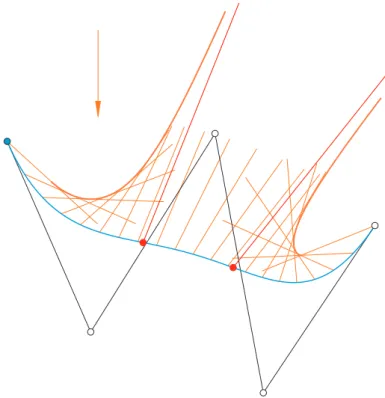
The caustic may have point(s) at infinity, i.e., the curve can be composed of several branches. This happens where the denominator 𝑟˙𝑥(𝑡) ¨𝑟𝑦(𝑡)−𝑟¨𝑥(𝑡) ˙𝑟𝑦(𝑡) vanishes, i.e., where the curvature ofr is zero. The asymptote at such a point is the reflected ray r(𝑡) +𝜆v(𝑡), 𝜆 ∈ R itself. In Fig. 1 there is a quartic Bézier curve the caustic of which has two points at infinity.

Figure 1: A quartic Bézier curve along with its caustic, which has two points at infinity. The arrow indicates the light direction.

(3)

From here on, we will study the caustics of planar Bézier curves r(𝑡) =

∑︁𝑛 𝑖=0

𝐵^𝑛_𝑖 (𝑡)b𝑖, 𝑡∈[0,1], 𝑛≥2,

where the sequence of points{b𝑖}^𝑛𝑖=0are called control points and𝐵_𝑖^𝑛 denotes the 𝑖th Bernstein polynomial of degree𝑛. (The case𝑛= 1is out of interest, since then the curve degenerates to a straight line segment and the reflected rays are parallel.)

3. Caustic of a Bézier curve

At first, we reformulate the caustic c to have a common denominator of the the coordinate functions, yielding

𝑐𝑥(𝑡) = 2 ( ˙𝑟𝑥(𝑡) ¨𝑟𝑦(𝑡)−¨𝑟𝑥(𝑡) ˙𝑟𝑦(𝑡))𝑟𝑥(𝑡) + ˙𝑟²_𝑥(𝑡) ˙𝑟𝑦(𝑡)−𝑟˙³_𝑦(𝑡)

2 ( ˙𝑟𝑥(𝑡) ¨𝑟𝑦(𝑡)−𝑟¨𝑥(𝑡) ˙𝑟𝑦(𝑡)) , (3.1) 𝑐𝑦(𝑡) = 2 ( ˙𝑟𝑥(𝑡) ¨𝑟𝑦(𝑡)−¨𝑟𝑥(𝑡) ˙𝑟𝑦(𝑡))𝑟𝑦(𝑡) + 2 ˙𝑟𝑥(𝑡) ˙𝑟_𝑦²(𝑡)

2 ( ˙𝑟𝑥(𝑡) ¨𝑟𝑦(𝑡)−¨𝑟𝑥(𝑡) ˙𝑟𝑦(𝑡)) . (3.2) Obviously, numerators of the above expressions are polynomials of degree3 (𝑛−1) and the common denominator is of degree (2𝑛−3), therefore these coordinate functions are rational functions of degree3 (𝑛−1). In what follows we provide the rational Bézier representation of such caustics. We introduce notations

˙r(𝑡) =

𝑛−1∑︁

𝑖=0

𝐵_𝑖^𝑛−1(𝑡)a𝑖, 𝑡∈[0,1], a𝑖=𝑛(b𝑖+1−b𝑖), 𝑖= 0,1, . . . , 𝑛−1,

¨r(𝑡) =

𝑛−2∑︁

𝑖=0

𝐵_𝑖^𝑛⁻²(𝑡)d𝑖, 𝑡∈[0,1], d𝑖= (𝑛−1) (a𝑖+1−a𝑖), 𝑖= 0,1, . . . , 𝑛−2.

Making use of the identity

𝐵_𝑖^𝑛(𝑡)𝐵_𝑗^𝑚(𝑡) = (︀𝑛

𝑖

)︀(︀𝑚 𝑗

)︀

(︀𝑛+𝑚 𝑖+𝑗

)︀𝐵_𝑖+𝑗^𝑛+𝑚(𝑡)

of Bernstein polynomials (cf. [1]), we can derive an identity for the product of two linear combinations∑︀𝑛

𝑖=0𝐵^𝑛_𝑖 (𝑡)𝑎𝑖 and∑︀𝑚

𝑗=0𝐵_𝑗^𝑚(𝑡)𝑏𝑗 can be written in the form

∑︁𝑛 𝑖=0

𝐵_𝑖^𝑛(𝑡)𝑎𝑖

∑︁𝑚 𝑗=0

𝐵_𝑗^𝑚(𝑡)𝑏𝑗=

𝑛+𝑚∑︁

ℓ=0

𝐵_ℓ^𝑛+𝑚(𝑡) 1 (︀𝑛+𝑚

ℓ

)︀

∑︁𝑚 𝑘=0

(︂ 𝑛 ℓ−𝑘

)︂(︂𝑚 𝑘

)︂

𝑎_ℓ−𝑘𝑏𝑘, (3.3) provided𝑛≥𝑚.

(4)

Now, we study the common denominator. By means of identity 3.3, its first term is of the form

˙

𝑟𝑥(𝑡) ¨𝑟𝑦(𝑡) =

𝑛−1

∑︁

𝑖=0

𝐵_𝑖^𝑛−1(𝑡)𝑎𝑥,𝑖 𝑛∑︁−2 𝑗=0

𝐵^𝑛−2_𝑗 (𝑡)𝑑𝑦,𝑗

=

2𝑛∑︁−3 ℓ=0

𝐵_ℓ^2𝑛−3(𝑡) 1 (︀2𝑛−3

ℓ

)︀

𝑛−2

∑︁

𝑘=0

(︂𝑛−1 ℓ−𝑘

)︂(︂𝑛−2 𝑘

)︂

𝑎𝑥,ℓ−𝑘𝑑𝑦,𝑘. The second term can analogously be expressed, yielding

˙

𝑟𝑦(𝑡) ¨𝑟𝑥(𝑡) =

2𝑛∑︁−3 ℓ=0

𝐵_ℓ^2𝑛⁻³(𝑡) 1 (︀_2𝑛−3

ℓ

)︀

𝑛−2

∑︁

𝑘=0

(︂𝑛−1 ℓ−𝑘

)︂(︂𝑛−2 𝑘

)︂

𝑎𝑦,ℓ−𝑘𝑑𝑥,𝑘

and the denominator has the form

2 ( ˙𝑟𝑥(𝑡) ¨𝑟𝑦(𝑡)−𝑟¨𝑥(𝑡) ˙𝑟𝑦(𝑡)) =

2𝑛−3∑︁

ℓ=0

𝑤ℓ𝐵_ℓ^2𝑛⁻³(𝑡), (3.4) where

𝑤ℓ= 2 (︀2𝑛−3

ℓ

)︀

𝑛−2

∑︁

𝑘=0

(︂𝑛−1 ℓ−𝑘

)︂(︂𝑛−2 𝑘

)︂

(𝑎𝑥,ℓ−𝑘𝑑𝑦,𝑘−𝑎𝑦,ℓ−𝑘𝑑𝑥,𝑘). (3.5) We elevate the degree of (3.4) by𝑛, using the general degree elevation formula

∑︁𝑠 𝑖=0

𝐵_𝑖^𝑠(𝑡)𝑤𝑖=

𝑠+𝑧∑︁

𝑖=0

𝐵^𝑠+𝑧_𝑖 (𝑡)𝑤^[𝑧]_𝑖 , 𝑧 >0, (3.6) 𝑤_𝑖^[𝑧]=𝑤^[𝑧−1]_𝑖 + 𝑖

𝑠+𝑧

(︁𝑤_𝑖^[𝑧−1]₋₁ −𝑤^[𝑧−1]_𝑖 )︁

, 𝑖= 0,1, . . . , 𝑠+𝑧 𝑤_𝑖^[0]=𝑤𝑖, 𝑖= 0,1, . . . , 𝑠.

with substitutions𝑠= 3 (𝑛−1) and𝑧=𝑛.

The degree elevated denominator is

3(𝑛−1)

∑︁

ℓ=0

𝑤^[𝑛]_ℓ 𝐵^3(𝑛_ℓ ⁻¹⁾(𝑡), 𝑡∈[0,1].

The numerator of the𝑥coordinate function is

2 ( ˙𝑟𝑥(𝑡) ¨𝑟𝑦(𝑡)−𝑟¨𝑥(𝑡) ˙𝑟𝑦(𝑡))𝑟𝑥(𝑡) + ˙𝑟_𝑥²(𝑡) ˙𝑟𝑦(𝑡)−𝑟˙_𝑦³(𝑡). Its first term can be expressed as

2 ( ˙𝑟𝑥(𝑡) ¨𝑟𝑦(𝑡)−𝑟¨𝑥(𝑡) ˙𝑟𝑦(𝑡))𝑟𝑥(𝑡)

(5)

=

3(𝑛−1)

∑︁

ℓ=0

𝐵_ℓ^3(𝑛⁻¹⁾(𝑡) 1 (︀3(𝑛−1)

ℓ

)︀

(︃ _𝑛

∑︁

𝑘=0

(︂2𝑛−3 ℓ−𝑘

)︂(︂𝑛 𝑘 )︂

𝑤ℓ−𝑘𝑏𝑥,𝑘

)︃

and the second one as

˙

𝑟_𝑥²(𝑡) ˙𝑟𝑦(𝑡) =

3(𝑛−1)

∑︁

ℓ=0

𝐵^3(𝑛−1)_ℓ (𝑡) 1 (︀_3(𝑛−1)

ℓ

)︀

×

𝑛∑︁−1 𝑘=0

(︃(︂𝑛−1 𝑘

)︂

𝑎𝑦,𝑘 𝑛∑︁−1 𝑧=0

(︂ 𝑛−1 ℓ−𝑘−𝑧

)︂(︂𝑛−1 𝑧

)︂

𝑎𝑥,ℓ−𝑘−𝑧𝑎𝑥,𝑧

)︃

while the third one as

˙ 𝑟³_𝑦(𝑡) =

3(𝑛−1)

∑︁

ℓ=0

𝐵_ℓ^3(𝑛−1)(𝑡) 1 (︀_3(𝑛−1)

ℓ

)︀

×

𝑛∑︁−1 𝑘=0

(︃(︂𝑛−1 𝑘

)︂

𝑎𝑦,𝑘 𝑛−1

∑︁

𝑧=0

(︂ 𝑛−1 ℓ−𝑘−𝑧

)︂(︂𝑛−1 𝑧

)︂

𝑎𝑦,ℓ−𝑘−𝑧𝑎𝑦,𝑧

)︃

. Thus, the numerator of Eq. (3.1) can be written in the form

3(𝑛−1)

∑︁

ℓ=0

𝐵_ℓ^3(𝑛⁻¹⁾(𝑡)𝑞𝑥,ℓ, where

𝑞𝑥,ℓ= 1 (︀3(𝑛−1)

ℓ

)︀

(︃ _𝑛

∑︁

𝑘=0

(︂2𝑛−3 ℓ−𝑘

)︂(︂𝑛 𝑘 )︂

𝑤ℓ−𝑘𝑏𝑥,𝑘+

𝑛−1

∑︁

𝑘=0

(︂𝑛−1 𝑘

)︂

𝑎𝑦,𝑘

×

𝑛−1∑︁

𝑧=0

(︂ 𝑛−1 ℓ−𝑘−𝑧

)︂(︂𝑛−1 𝑧

)︂

(𝑎_{𝑥,ℓ−𝑘−𝑧}𝑎𝑥,𝑧−𝑎_{𝑦,ℓ−𝑘−𝑧}𝑎𝑦,𝑧) )︃

. (3.7)

Analogously, we can obtain the numerator of (3.2) in the form

3(𝑛−1)

∑︁

ℓ=0

𝐵_ℓ^3(𝑛⁻¹⁾(𝑡)𝑞𝑦,ℓ,

where

𝑞𝑦,ℓ= 1 (︀3(𝑛−1)

ℓ

)︀

(︃ _𝑛

∑︁

𝑘=0

(︂2𝑛−3 ℓ−𝑘

)︂(︂𝑛 𝑘 )︂

𝑤ℓ−𝑘𝑏𝑦,𝑘+ 2

𝑛−1

∑︁

𝑘=0

(︂𝑛−1 𝑘

)︂

𝑎𝑥,𝑘

×

𝑛−1∑︁

𝑧=0

(︂ 𝑛−1 ℓ−𝑘−𝑧

)︂(︂𝑛−1 𝑧

)︂

𝑎_{𝑦,ℓ−𝑘−𝑧}𝑎𝑦,𝑧

)︃

. (3.8)

(6)

Finally, the rational Bézier representation of the caustic curve is

c(𝑡) =

3(𝑛−1)∑︁

ℓ=0

𝑤^[𝑛]_ℓ 𝐵_ℓ^3(𝑛−1)(𝑡)

∑︀3(𝑛−1)

𝑘=0 𝑤_𝑘^[𝑛]𝐵_𝑘^3(𝑛⁻¹⁾(𝑡)qℓ, 𝑡∈[0,1]

where weights{︁

𝑤_ℓ^[𝑛]}︁3(𝑛−1)

ℓ=0 are the coefficients obtained by the degree elevation of the denominator, and control points are specified by

qℓ= 1 𝑤_ℓ^[𝑛]

[︂ 𝑞𝑥,ℓ

𝑞𝑦,ℓ

]︂

, ℓ= 0,1, . . . ,3 (𝑛−1). (3.9)

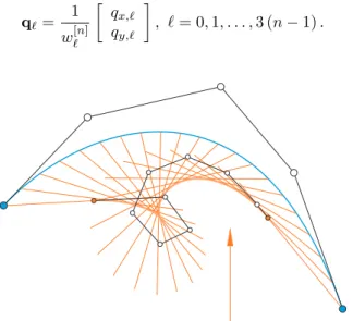
Figure 2: A quartic Bézier curve and its caustic along with the reflected rays. The control polygon of the rational Bézier representation (which is of degree9) is also displayed. The arrow indicates

the light direction.

Now, we summarize our results.

Proposition 3.1. The caustic of a Bézier curve of degree𝑛(if exists) is a rational Bézier curve of degree3 (𝑛−1). Its weights and control points are specified by(3.5), (3.6)and (3.7),(3.8),(3.9), respectively.

Remark 3.2. The caustic of a quadratic Bézier curve(𝑛= 2)(if exists) is a cubic polynomial curve, since in this case the common denominator of (3.1) and (3.2) is the constant

∑︁1 ℓ=0

𝐵_ℓ¹(𝑡) (︃

2

∑︁1 𝑘=0

(︀2−1 ℓ−𝑘

)︀(︀0 𝑘

)︀

(︀1 ℓ

)︀ (𝑎𝑥,ℓ−𝑘𝑑𝑦,𝑘−𝑎𝑦,ℓ−𝑘𝑑𝑥,𝑘) )︃

= 2

∑︁1 ℓ=0

𝐵_ℓ¹(𝑡) (𝑎𝑥,ℓ𝑑𝑦,0−𝑎𝑦,ℓ𝑑𝑥,0)

(7)

= 2 (𝑎𝑥,0𝑎𝑦,1−𝑎𝑥,1𝑎𝑦,0)(︀

𝐵¹₀(𝑡) +𝐵₁¹(𝑡))︀

= 2 (𝑎𝑥,0𝑎𝑦,1−𝑎𝑥,1𝑎𝑦,0),

therefore the caustic is a cubic polynomial curve. It is well-known that the caustic of a parabola is a Tschirnhausen cubic, if the rays are not parallel to the axis of the parabola, we have just obtained its Bézier representation.

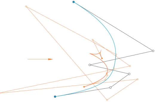
Figure 3: A quintic Bézier curve the caustic of which has two cusps. The control polygon of the rational Bézier representation of the caustic is also shown. The arrow indicates the light direction.

Remark 3.3. The cusp(s) of the caustic may be of interest. The causticchas a cusp at 𝑡0∈ [0,1], if ‖c˙(𝑡0)‖ = 0, i.e., if the tangent vector vanishes, that we can find numerically. Actually, it is a root finding problem, which can be solved efficiently with high precision and stability, since the polynomials are specified in Bernstein basis (cf. [2, 5]).

In Fig. 2 there is a quartic Bézier curve and its caustic, along with the control polygon of the rational Bézier representation of the caustic. Fig. 3 shows such a quintic Bézier curve whose caustic has two cusps.

4. Conclusions

We have provided ready to implement exact formulae for the rational Bézier representation of caustics (if exist) of planar Bézier curves of degree greater than

(8)

one. This method can be extended to other control point based curves, i.e., curves described in the form

c(𝑡) =

∑︁𝑛 𝑖=0

𝐹_𝑖^𝑛(𝑡)d𝑖, 𝑡∈[𝑎, 𝑏].

We assume that function system ℱ := {𝐹𝑖|𝐹𝑖: [𝑎, 𝑏]→R}^𝑛𝑖=0 consists of sufficiently smooth non-negative functions, forming a partition of unity. Additional requirements are the existence of degree elevation and product formulae in the ba- sisℱ. These requirements are fulfilled by the B-basis of trigonometric (cf. [3]) and that of hyperbolic polynomials (cf. [4]), besides the Bernstein basis.

References

[1] G. Farin:Curves and surfaces for CAGD: a practical guide, 5th edition, Morgan Kaufmann, 2001,doi:10.1016/B978-1-55860-737-8.X5000-5.

[2] R. T. Farouki,V. Rajan:Algorithms for polynomials in Bernstein form, Computer Aided Geometric Design 5.1 (1988), pp. 1–26,doi:10.1016/0167-8396(88)90016-7.

[3] J. Sánchez-Reyes:Harmonic rational Bézier curves, p-Bézier curves and trigonometric polynomials, Computer Aided Geometric Design 15.9 (1998), pp. 909–923, doi:10 . 1016 / S0167-8396(98)00031-4.

[4] W.-Q. Shen,G.-Z. Wang:A class of quasi Bézier curves based on hyperbolic polynomials, Journal of Zhejiang University Science 6.1 (2005), pp. 116–123,doi:10.1007/BF02887226.

[5] M. R. Spencer:Polynomial real root finding in Bernstein form, PhD thesis, Brigham Young University, 1994,url:https://scholarsarchive.byu.edu/etd/4246.

[6] E. Troll,M. Hoffmann:Caustics of spline curves, Annales Mathematicae et Informati- cae 47 (2017), pp. 201–209, url:http://ami.ektf.hu/uploads/papers/finalpdf/AMI%

5Ctextunderscore47%5Ctextunderscore%20from201to209.pdf.