On the generalization of Erdos-Vincze’s theorem about the approximation of regular triangles by polyellipses in the plane

On the generalization of Erdős-Vincze’s theorem about the approximation of regular triangles by polyellipses in the plane

Cs. Vincze

, Z. Kovács

, Zs. F. Csorvássy

aInstitute of Mathematics, University of Debrecen, P.O.Box 400, H-4002 Debrecen, Hungary

csvincze@science.unideb.hu

bInstitute of Mathematics and Computer Science, University of Nyíregyháza, H-4400 Nyíregyháza, Sóstói út 31./B, Hungary

kovacs.zoltan@nye.hu

cDebrecen Reformed Theological University, H-4026 Debrecen, Kálvin tér 16, Hungary csorvassy.zs.f@gmail.com

Submitted September 26, 2017 — Accepted May 29, 2018 Dedicated to Professor Lajos Tamássy on his 95th birthday.

Abstract

A polyellipse is a curve in the Euclidean plane all of whose points have the same sum of distances from finitely many given points (focuses). The classical version of Erdős-Vincze’s theorem states that regular triangles can not be presented as the Hausdorff limit of polyellipses even if the number of the focuses can be arbitrary large. In other words, the topological closure of the set of polyellipses with respect to the Hausdorff distance does not contain any regular triangle, and we have a negative answer to the problem posed by E. Vázsonyi (Weissfeld) about the approximation of closed convex plane curves by polyellipses. It is the additive version of the approximation of simple closed plane curves by polynomial lemniscates all of whose points have the

∗Cs. Vincze is supported by the EFOP-3.6.1-16-2016-00022 project. The project is co-financed by the European Union and the European Social Fund.

doi: 10.33039/ami.2018.05.003 http://ami.uni-eszterhazy.hu

181

same product of distances from finitely many given points (focuses). Here we are going to generalize the classical version of Erdős-Vincze’s theorem for regular polygons in the plane. We will conclude that the error of the approximation tends to zero as the number of the vertices of the regular polygon tends to the infinity. The decreasing tendency of the approximation error gives the idea to construct curves in the topological closure of the set of polyellipses. If we use integration to compute the average distance of a point from a given (focal) set in the plane, then the curves all of whose points have the same average distance from the focal set can be given as the Hausdorff limit of polyellipses corresponding to partial sums.

Keywords:Polyellipses, Hausdorff distance, Generalized conics MSC:51M04

1. Introduction

Polyellipses in the plane belong to the more general idea of generalized conics [7], [8], [9], see also [3]. They are subsets all of whose points have the same average distance from a given set of points (focal set). The level set of the function measuring the arithmetic mean of Euclidean distances from the elements of a finite pointset is one of the most important discrete cases. Curves given by equation

Xm i=1

d(X, Fi) =c ⇔ Pm

i=1d(X, Fi)

m =cm (cm:=c/m) (1.1) are called polyellipses with focuses F1, . . . , Fm, where dmeans the Euclidean dis- tance in the plane. They are the additive version of lemniscates all of whose points have the same geometric mean of distances (i.e. their product is constant). Polyel- lipses appear in optimization problems in a natural way [5]. The characterization of the minimizer of a function measuring the sum of distances from finitely many given points is due to E. Vázsonyi (Weissfeld) [10]. He also posed the problem of the approximation of closed convex plane curves with polyellipses. P. Erdős and I. Vincze [1] proved that it is impossible in general because regular triangles can not be presented as the Hausdorff limit of polyellipses, even if the number of the focuses can be arbitrary large. The proof of the classical version of Erdős-Vincze’s theorem can be also found in [6]. The aim of the present paper is to generalize the theorem for regular polygons. Although a more general theorem can be found in P. Erdős and I. Vincze [2] stating that the limit shape of a sequence of polyellipses may have only one single straight segment, the high symmetry of regular polygons allows us to follow a special argument based on the estimation of the curvature of polyellipses with high symmetry. On the other hand, we conclude that the error of the approximation is tending to zero as the number of the vertices of the regular polygon tends to the infinity. The decreasing tendency of the approximation error gives the idea to construct curves in the topological closure of the set of polyellipses.

If we use integration to compute the average distance of a point from a given (focal)

set in the plane, then the curves all of whose points have the same average distance from the focal set can be given as the Hausdorff limit of polyellipses corresponding to partial sums. The idea can be found in [2], but it was formulated by some other authors as well, see e.g. [3].

Definition 1.1. LetR >0 be a positive real number. Theparallel body KR of a setK with radiusRis the union of the closed disks with radiusRcentered at the points ofK. The infimum of the positive numbers such that Lis a subset of the parallel body ofK with radius R, and vice versa, is called theHausdorff distance ofK andL, i.e.

h(K, L) = inf{R >0 |L⊂KR, K⊂LR}.

It is well-known that the Hausdorff metric makes the family of nonempty closed and bounded (i.e. compact) subsets in the plane a complete metric space. Another possible characterization of the Hausdorff distance between compact subsets can be given in terms of distances between the points of the sets: if

maxX∈Kd(X, L) := max

X∈Kmin

Y∈Ld(X, Y) and max

Y∈Ld(K, Y) := max

Y∈L min

X∈Kd(X, Y), then the Hausdorff distance of KandL is

h(A, B) = max{max

X∈Kd(X, L),max

Y∈Ld(K, Y)}. (1.2)

2. Polyellipses in the Euclidean plane

Definition 2.1. Let F1, . . . , Fm be not necessarily different points in the plane and consider the function

F(X) :=

Xm i=1

d(X, Fi)

measuring the sum of distances ofX fromF1, . . . , Fm. The set given by equation F(X) =c is called a polyellipse with focuses F1, . . . , Fm. The multiplicity of the focal pointFi (i= 1, . . . , m)is the number of its appearances in the sum.

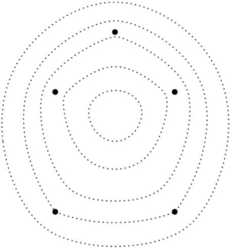
2.1. A Maple presentation I

with(plottools):

with(plots):

#The coordinates of the focal points#

x:=[0.,1.,1.,0.,.5]:

y:=[0.,0.,1.,1.,1.5]:

m:=nops(x):

F:=proc(u,v) local i,partial:

partial:=0.:

for i to m do

partial:=partial+sqrt((u-x[i])^2+(v-y[i])^2) end do

end proc:

#The list of the level rates#

c:=[3.75,4,4.5,5,5.7]:

graf1:=pointplot(zip((s,t)->[s,t],x,y),symbol=solidcircle, symbolsize=20, color=black):

graf2:=

seq(implicitplot(F(u,v)=i,u=-2..2,v=-2..2,numpoints=10000, color=black), i=c):

display(graf1,graf2,scaling=constrained,axes=none,linestyle=dot);

Figure 1: A Maple presentation I

2.2. Weissfeld’s theorems

Using the triangle inequality, it is easy to prove thatF is a convex function; more- over if the focuses are not collinear, then it is strictly convex. It is also clear that F is differentiable at each point different from the focuses and

DvF(X) =hv, Ni, where N :=− Xm i=1

1 d(X, Fi)

XF−→i (2.1)

is the opposite vector of the sum of unit vectors from X to the focal points, re- spectively. Using that the vanishing of the first order derivatives is a sufficient and necessary condition for a point to be the minimizer of a convex function, we have the first characterization theorem due to E. Vázsonyi (Weissfeld).

Theorem 2.2 ([10]). Suppose that X is different from the focal points; it is a minimizer of the function F if and only if

N =0 ⇔ Xm i=1

1 d(X, Fi)

XF−→i=0.

A more subtle, but standard convex analysis shows that if X =Fi is one of the focal points, then

D⁺_vF(Fi) =kikvk+hv, Nii,

where D⁺_vF(Fi) denotes the one-sided directional derivative of F at Fi into di- rection v (the one-sided directional derivatives always exist in case of a convex function),

Ni:=− X

Fj6=Fi

1 d(Fi, Fj)

F−→iFj

and ki is the multiplicity of the focal point Fi. Using that D⁺_vF(Fi) ≥ 0 for any direction v is a sufficient and necessary condition forFi to be the minimizer of the function F, the Cauchy-Buniakovsky-Schwarz inequality gives the second characterization theorem due to E. Vázsonyi (Weissfeld).

Theorem 2.3 ([10]). The focal pointX =Fi (i= 1, . . . , m)is a minimizer of the functionF if and only if

kNik ≤ki ⇔ k X

Fj6=Fi

1 d(Fi, Fj)

F−→iFjk ≤ki.

In terms of coordinates we have the following formulas:

D1F(x, y) = Xm i=1

x−xi

p(x−xi)²+ (y−yi)², (2.2)

D2F(x, y) = Xm i=1

y−yi

p(x−xi)²+ (y−yi)²

provided thatX(x, y)is different from the focuses Fi(xi, yi), where i = 1, . . . , m.

The second order partial derivatives are D1D1F(x, y) =

Xm i=1

(y−yi)²

((x−xi)²+ (y−yi)²)^3/2, D2D2F(x, y) =

Xm i=1

(x−xi)²

((x−xi)²+ (y−yi)²)^3/2, (2.3) D1D2F(x, y) =−

Xm i=1

(x−xi)(y−yi) ((x−xi)²+ (y−yi)²)^3/2.

2.3. The main theorem

The classical version of Erdős-Vincze’s theorem states that regular triangles can not be presented as the Hausdorff limit of polyellipses, even if the number of the focuses can be arbitrary large, and we have a negative answer to the problem posed by E.

Vázsonyi about the approximation of closed convex planar curves by polyellipses.

It is the additive version of the approximation of simple closed planar curves by polynomial lemniscates all of whose points have the same product of distances from finitely many given points¹(focuses). Here we are going to generalize the classical version of Erdős-Vincze’s theorem for any regular polygon in the plane as follows.

Theorem 2.4. A regular p- gon(p≥3)in the plane can not be presented as the Hausdorff limit of polyellipses, even if the number of the focuses can be arbitrary large.

3. The proof of Theorem 3

Let P be a regular p - gon with vertices P1, . . . , Pp inscribed in the unit circle centered at the point O and suppose, in contrary, that there is a sequence En of polyellipses tending toP.

3.1. The first step: the reformulation of the problem by cir- cumscribed polyellipses.

Letε >0 be an arbitrarily small positive real number and suppose thatnis large enough forEnto be contained in the ring of the circlesC₋εandCεaroundO with radiuses1−εand 1 +ε. IfP₋εis the regularp- gon inscribed inC₋εthenEn is a polyellipse aroundP₋ε. On the other hand,

h(P₋ε, En)≤h(P₋ε, P) +h(P, En)≤ε+h(C₋ε, Cε) = 3ε.

Using a central similarity with centerO and coefficient ₁₋¹_ε, we have that P₋ε7→

P₋⁰_ε=P andEn 7→E_n⁰, whereE_n⁰ is a polyellipse aroundP such that h(P, E_n⁰) =h(P_−ε⁰ , E_n⁰) = 1

1−εh(P₋ε, En)≤ 3ε 1−ε.

Takingε→0 we have a sequence of circumscribed polyellipses tending toP. 3.1.1. Summary

From now on, we suppose that En is a sequence of circumscribed polyellipses tending to P.

1The approximating process uses the partial sums of the Taylor expansion of holomorphic functions and the focuses correspond to the complex roots of the polynomials.

3.2. The second step: a symmetrization process.

Following the basic idea of [1], we apply a symmetrization process to the circum- scribed polyellipses ofPwithout increasing the Hausdorff distances. LetF1, . . . , Fm

be the focuses of a polyellipseE aroundP defined by the formula Xm

i=1

d(X, Fi) =c.

Consider the polyellipse Esym passing through the verticesP1, . . . , Pp of P such that its focal set is

G:={f(Fi)|i= 1, . . . , mandf ∈H}, (3.1) whereH denotes the symmetry group ofP. The equation ofEsymis

X

f∈H

Xm i=1

d(X, f(Fi)) =c⁰,

where c⁰:= X

f∈H

Xm i=1

d(P1, f(Fi)) = X

f∈H

Xm i=1

d(P2, f(Fi)) =. . .= X

f∈H

Xm i=1

d(Pp, f(Fi)) because of the invariance of the vertices and the focal set under the groupH. Note that f(E)is a polyellipse around P with focusesf(F1), . . ., f(Fm). It is defined by the equation

Xm i=1

d(X, f(Fi)) =c and h(P, f(E)) =h(f(P), f(E)) =h(P, E) (3.2) because P is invariant underf for any f ∈H. Then, for example,

Xm i=1

d(P1, f(Fi))≤c.

Taking the sum asf runs through the elements of H we have that c⁰ ≤2pc. On the other hand, ifX is an outer point off(E)for any f ∈H, then

Xm i=1

d(X, f(Fi))> c (f ∈H), i.e. X

f∈H

Xm i=1

d(X, f(Fi))>2pc≥c⁰. By contraposition, if X belongs to the polyellipse Esym, then it belongs to the convex hull off(E)forsome f ∈H. Finally,

Esym⊂ [

f∈H

convf(E),

where conv f(E) denotes the convex hull of the polyellipse f(E) (f ∈H). Since each polyellipse is aroundP, it follows that

h(P, Esym)≤h



P, [

f∈H

convf(E)



≤h



P, [

f∈H

f(E)



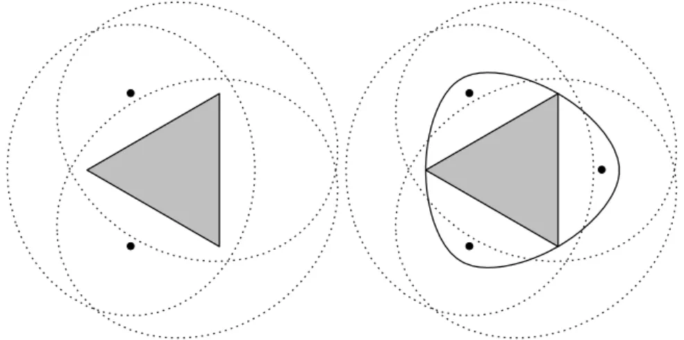
=h(P, E) because the possible distances between the points of the sets P and f(E) are independent of the choice of f ∈ H (see the minimax characterization (1.2) of the Hausdorff distance). Figure 2 (left hand side) illustrates an ellipse E with focuses F1, F2 and its symmetric pairs with respect to the isometry group of the triangle (p= 3). The focal set of E_sym (right hand side) contains three different pointsF1, F2, F3 (solidcircles) with multiplicityk1=k2=k3= 2. The constant is choosen such thatE_sym passes through the vertices of the polygon.

Figure 2: The symmetrization process

3.2.1. Summary

From now on, we suppose that En is a sequence of circumscribed polyellipses tending to P such that each element of the sequence passes through the vertices P1, . . . , Pp ofP, and the set of the focuses is of the form (3.1).

3.3. The third step - smoothness.

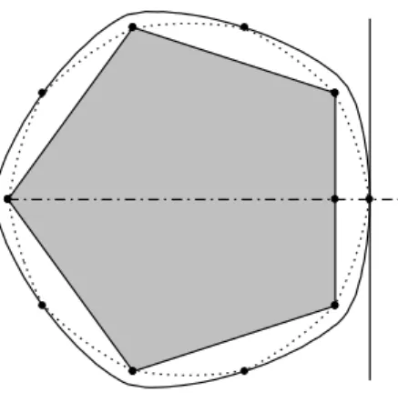
By the symmetry properties it can be easily seen that h(P, E) =d(Mi, Qi) (i= 1, . . . p),

whereEstands for a general element of the sequence of polyellipses,MiandQiare the corresponding midpoints of the edge² PiPi+1 of P and the arc PiPi+1 of the

2The indices are taken by modulop.

polyellipse, respectively. Note that the line passing throughQiparallel to the edge PiPi+1of the polygon supports the polyellipse at Qi because of the symmetry, see Figure 3. For the sake of simplicity consider the case ofi= 1and

Q:=Q1, M:=M1.

It is clear that the polyellipse E heritages the symmetries of its focal set, i.e. E is invariant under the reflection about the horizontal line. So are the supporting lines atQ. Therefore the line passing throughQparallel to the edgeP1P2 of the polygon supports the polyellipse atQ.

Since the next step of the proof will be the estimation of the curvature of the polyellipse E at the point Q, but a polyellipse can pass through some of its focuses (see Figure 1), we need an extra process to avoid singularities. Consider the equation

X

f∈H

Xm i=1

d(X, f(Fi)) =c

of the polyellipseE, where

c:= X

f∈H

Xm i=1

d(P1, f(Fi)) = X

f∈H

Xm i=1

d(P2, f(Fi)) =. . .= X

f∈H

Xm i=1

d(Pp, f(Fi))

and suppose thatF1=Qsuch that X

f∈H

Xm i=1

d(Q, f(Fi)) =c.

Then X

f∈H

X

Fi=Q

d(Q, f(Q)) +X

f∈H

X

Fi6=Q

d(Q, f(Fi)) =c,

k1

X

f∈H

d(Q, f(Q)) +X

f∈H

X

Fi6=Q

d(Q, f(Fi)) =c (3.3) and, because ofP1∈E,

k1

X

f∈H

d(P1, f(Q)) +X

f∈H

X

Fi6=Q

d(P1, f(Fi)) =c. (3.4) Consider the function

F(X) := X

f∈H

d(X, f(M));

using the triangle inequality, it can be easily seen thatFis a strictly convex function such that

F(P1) =. . .=F(Pn).

Figure 3: Smoothness

ThereforeF(M)< F(P1)becauseM is the midpoint of the segmentP1P2. IfQis close enough toM then

X

f∈H

d(Q, f(Q))≈F(M)< F(P1)≈ X

f∈H

d(P1, f(Q))

by a continuity argument. Therefore, equations (3.3) and (3.4) show that c⁰:= X

f∈H

X

Fi6=Q

d(Q, f(Fi))>X

f∈H

X

Fi6=Q

d(P1, f(Fi)).

Now the polyellipseE⁰ defined by X

f∈H

X

Fi6=Q

d(X, f(Fi)) =c⁰

passes through Q but P1 and, by the symmetry,P2 are in the interior of E⁰ (see Figure 3). SinceQ(together with all symmetric pairs) has been deleted from the focal points, we can take the curvature κofE⁰ at Q:

κ(Q)≤ 1

the radius of the circle passing throughP1, P2andQ.

In case of a sequence of polyellipses tending to P, the point Q can be arbitrarily close toM, and κ(Q)can be arbitrarily close to zero.

3.4. The estimation of the curvature

From now on, we suppose that the set of the focuses of the polyellipse E is of the form (3.1) and Q is the corresponding point on the arc of the polyellipse to the midpointM of the edgeP1P2. To simplify the curvature formula [4] atQas far as possible, suppose that

P1(cos(π/p),−sin(π/p)), P2(cos(π/p),sin(π/p)) and M(cos(π/p),0),

i.e. the tangent line to the polyellipse at Qis parallel to the y - axis. Therefore D2F(Q) = 0,where

F(X) = X

f∈H

Xm i=1

d(X, f(Fi)) and κ(Q) =D2D2F(Q)

D1F(Q) . (3.5) SinceD1F(Q)is the first coordinate of the gradient vector ofF atQ, we have from (2.1) that

0< D1F(Q) =kX

f∈H

Xm i=1

1 d(Q, f(Fi))

−→

Qf(Fi)k ≤

2pk0+kX

f∈H

X

Fi6=O

1 d(Q, f(Fi))

Qf−→(Fi)k,

where k0 is the multiplicity of the symmetry center O if it belongs to the set of focusesF1, . . .,Fm, andk0= 0otherwise. Applying Theorem 2.2 to the function

F0(X) := X

f∈H

X

Fi6=O

d(X, f(Fi)), it follows that

X

f∈H

X

Fi6=O

1 d(O, f(Fi))

Of−→(Fi)=0.

Therefore

0< D1F(Q) =kX

f∈H

Xn i=1

1 d(Q, f(Fi))

Qf(F−→i)k ≤

2pk0+kX

f∈H

X

Fi6=O

1 d(Q, f(Fi))

−→

Qf(Fi)k=

2pk0+kX

f∈H

X

Fi6=O

1 d(Q, f(Fi))

−→

Qf(Fi)−X

f∈H

X

Fi6=O

1 d(O, f(Fi))

−→

Of(Fi)k ≤

2pk0+X

f∈H

X

Fi6=O

k 1 d(Q, f(Fi))

Qf−→(Fi)− 1 d(O, f(Fi))

Of(F−→i)k.

Lemma 3.1. If Qis close enough to M then k 1

d(Q, f(Fi))

Qf(F−→i)− 1 d(O, f(Fi))

Of−→(Fi)k ≤ 4 1 +d(O, Fi) for any Fi 6=O,i= 1, . . . , m.

Proof. IfFi is in the interior of the unit circle centered atO, then the same is true for any point of the form f(Fi) because O is the fixpoint of the elements in the symmetry group H. Therefore

4

1 +d(O, Fi)≥ 4 1 + 1 = 2

which is the maximum of the length of the difference of unit vectors. Otherwise, if Fi (together with its all symmetric pairs) is an outer point of the unit circle centered at O and Q is in its interior, i.e. Q is close enough to M, then αi :=

∠(Of(Fi)Q)<90^◦ for anyf ∈H. By the cosine rule k 1

d(Q, f(Fi))

Qf−→(Fi)− 1 d(O, f(Fi))

Of−→(Fi)k²= 2(1−cosαi) = 4 sin²αi

2 , i.e.

k 1 d(Q, f(Fi))

−→

Qf(Fi)− 1 d(O, f(Fi))

−→

Of(Fi)k= 2 sinαi

2 ≤2 sinαi

because of 0≤αi<90^◦. By the sine rule

d(O, Fi) sinαi≤d(O, Q)<1 ⇒ sinαi< 2 1 +d(O, Fi) and the proof is complete.

Corollary 3.2.

0< D1F(Q1)≤2pk0+ 8p X

Fi6=O

1

1 +d(O, Fi) ≤8p Xm i=1

1 1 +d(O, Fi). Lemma 3.3. If Qis close enough to M then

D2D2(Q)≥2 cos²π p

Xm i=1

1 1 +d(O, Fi),

Proof. Using formula (2.3) we should estimate expressions of type S(Q, Fi) := X

f∈H

1

d(Q, f(Fi))cos²βi (3.6) for anyi= 1, . . . , m, where βi=∠(FiQO). By the triangle inequality

d(Q, f(Fi))≤d(Q, O) +d(O, f(Fi))≤1 +d(O, Fi)

provided that Qis in the interior of the unit circle centered at O, i.e. Q is close enough toM. Therefore

1 1 +d(O, Fi)

X

f∈H

cos²βi≤S(Q, Fi). (3.7)

First of all consider the case ofFi=O. By (3.7) S(Q, O)≥ X

f∈H

1 = 2p≥2 cos²π p

1

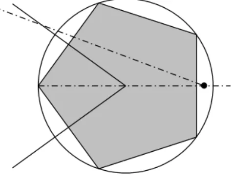
1 +d(O, O). (3.8) Suppose thatFi6=O. Since the focal set contains all symmetric pairs of Fi under the action of the elements inH, there must be at least two focal points of the form f(Fi) in the sector of the plane with polar angle between π−π/p and π+π/p (one of them as a rotated and another one as a reflected pair of Fi), see Figure 4.

Therefore

Figure 4: The proof of Lemma 2

S(Q, Fi)≥ 1 1 +d(O, Fi)

X

f∈H

cos²βi≥2 cos²π p

1

1 +d(O, Fi) (3.9) as was to be proved.

Using the curvature formula (3.5), Corollary 3.2 and Lemma 3.3 give that

κ(Q)≥cos^2π_p

4p , (3.10)

independently of the number of focuses. Therefore κ(Q) can not be arbitrarily close to zero which is a contradiction.

4. Concluding remarks

To present a reach class of curves in the plane as Hausdorff limits of polyellipses we should use integration to compute the average distance of a point from a given (focal) set. Let Γ be a plane curve with finite arclength L(Γ) and consider the function

f(X) := 1 L(Γ)

Z

Γ

d(X, Y)dY. (4.1)

The curve given by the equationf(X) =cis called a generalized conic with focal set Γ. In what follows we show that such a curve is the Hausdorff limit of polyellipses.

First of all note that f is convex because of the convexity of the integrand. This means that it is a continuous function, i.e. the level set f⁻¹(c)is closed. On the other hand it is bounded becauseΓis bounded. Therefore a generalized conic is a compact subset in the plane. Let ε >0 be a given positive number and consider the partition ofΓ into2^mequal parts (depending onX) such that

0< S(X, m)−s(X, m)< L(Γ)ε

2, (4.2)

whereX ∈f⁻¹(c),S(X, m)ands(X, m)are the upper and lower Riemann sum of Z

Γ

d(X, Y)dY

belonging to the equidistant partition. By a continuity argument³ formula (4.2) holds on an open disk centered X with radius rX. Since f⁻¹(c) is compact we can find a finite open covering with open disks centered at some points X1, . . ., Xk∈f⁻¹(c). Let

m:= max{m1, . . . , mk},

wheremidenotes the power of the partition of Γinto2^mi equal parts. Obviously, we have a refinement of all partitions under the choice of the maximal value of mi’s. Therefore

0< S(X, M)−s(X, M)< L(Γ)ε

2 (4.3)

for anyX∈f⁻¹(c), whereM := 2^m. Letτ1,. . .,τM ∈Γbe some middle points of the partition and define the function

FM(Z) :=d(Z, τ1) +. . .+d(Z, τM)

M . (4.4)

Since we have an equidistant partition it follows that 1

L(Γ)s(X, M)≤FM(X)≤ 1

L(Γ)S(X, M) ⇒ |FM(X)−c|< ε (4.5) for any X ∈f⁻¹(c). This means that f⁻¹(c) is between the polyellipses defined by the equationsFM(X) =c−εandFM(X) =c+ε, i.e. {X|FM(X) =c−ε} ⊂ f⁻¹(c) ⊂ {X|FM(X) = c+ε}. Taking the limit ε → 0 the sequences of the polyellipses on both the left and the right hand sides of the previous formula tends tof⁻¹(c).

3Recall that both the sup-function and the inf-function are Lipschitzian:

infξ d(X, ξ)≤inf

ξ d(X, Y) +d(Y, ξ) =d(X, Y) + inf

ξ d(Y, ξ), i.e. |inf_ξd(X, ξ)−inf_ξd(Y, ξ)| ≤d(X, Y).In a similar way,

sup

ξ

d(X, ξ)≤sup

ξ

d(X, Y) +d(Y, ξ) =d(X, Y) + sup

ξ

d(Y, ξ).

4.1. A Maple presentation II

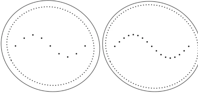
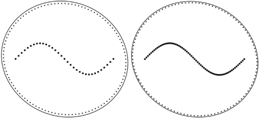
Since it is hard to find the equidistant partition of a curve in general, we use the equidistant partition of the parameter interval to present an explicite example: let Γ : γ: [0,2π] → γ(t) = (t,sin(t)) be a period of the sine wave. Figures 5 and 6 show the generalized conic f⁻¹(4) in "dot" linestyle (see equation (4.1)). The approximating polyellipses belong to the equidistant partition of the interval into M = 2³, 2⁴,2⁵ and2⁶equal parts, respectively.

Figure 5: A Maple presentation II: the case ofM = 2³and2⁴

with(plottools):

with(plots):

#The coordinates of the focal points#

x:=[seq((2*Pi*(1/8))*k,k=0..8)]:

y:=[seq(sin((2*Pi*(1/8))*k),k=0..8)]:

m:=nops(x):

F:=proc(u,v) local i,partial:

partial:=0.:

for i to m do

partial:=partial+\frac{1}{m}sqrt((u-x[i])^2+(v-y[i])^2) end do

end proc:

#The list of the level rates#

c:=[4]:

graf1:=pointplot(zip((s,t)->[s,t],x,y),symbol=solidcircle, symbolsize=10, color=black):

graf2:=seq(implicitplot(F(u,v)=i,u=-2..8,v=-5..5, numpoints=10000,color=black),i=c):

#Integration along the sine wave#

F:=(u,v)->(1/4)*Int(sqrt((u-t)^2+(v-sin(t))^2)*

sqrt(1+cos(t)^2),t=0..2*Pi)/(sqrt(2)*EllipticE((1/2)*sqrt(2))):

graf3:=implicitplot(F(u,v)=4,u=-2..8,v=-5..5,linestyle=dot, thickness=3,color=black):

display(graf1,graf2,graf3,scaling=constrained,axes=none);

Figure 6: A Maple presentation II: the case ofM = 2⁵and2⁶

4.2. A note about the error of the approximation of a regular polygon by polyellipses

IfΓis the unit circle in the plane thenf⁻¹(c)is invariant under any element of the isometry group because the level sets heritage the symmetries of the integration domain (focal set). Therefore f⁻¹(c) is a circle centered at the same point as Γ. Especially, Γ = f⁻¹(c), where c = 4/π. This means that the error of the approximation of a regular polygon by polyellipses tends to zero as the number of the vertices tends to the infinity: ifP is a regularp- gon inscibed in the unit circle Γ, then

h(P,Γ) = 1−cosπ

p and h(P, E)≤h(P,Γ) +h(Γ, E)≤1−cosπ p+ε provided thatE is an approximating polyellipse ofΓ with error less thenε.

References

[1] Erdős, P. and Vincze, I., On the approximation of closed convex plane curves, Mat. Lapok 9(1958), 19–36 (in Hungarian, summaries in Russian and German).

[2] Erdős, P. and Vincze, I., On the approximation of convex, closed plane curves by multifrocal ellipses, Essays in statistical science,J. Appl. Probab. Spec.Vol.19A (1982), 89–96.

https://doi.org/10.1017/s0021900200034483

[3] Gross, C. and Strempel, T.-K., On generalizations of conics and on a gener- alization of the Fermat-Toricelli problem, Amer. Math. Monthly, 105 (1998), no. 8,

732–743.

https://doi.org/10.1080/00029890.1998.12004955

[4] Goldman, R., Curvature formulas for implicite curves and surfaces,Computer Aided Geometric Design 22(2005), 632–658.

https://doi.org/10.1016/j.cagd.2005.06.005

[5] Melzak, Z. A. and Forsyth, J. S., Polyconics 1. Polyellipses and optimization, Quart. Appl. Math.35, Vol. 2 (1977), 239–255.

https://doi.org/10.1090/qam/448883

[6] Vincze, Cs. and Varga, A., On a lower and upper bound for the curvature of ellipses with more than two foci,Expo. Math.26(2008), 55–77.

https://doi.org/10.1016/j.exmath.2007.06.003

[7] Vincze, Cs. and Nagy, Á., Examples and notes on generalized conics and their applications,AMAPN Vol.26(2010), 359–575.

[8] Vincze, Cs. and Nagy, Á., An introduction to the theory of generalized conics and their applications,Journal of Geom. and Phys.Vol.61(2011), 815–828.

https://doi.org/10.1016/j.geomphys.2010.12.003

[9] Vincze, Cs. and Nagy, Á., On the theory of generalized conics with applications in geometric tomography,J. of Approx. Theory 164(2012), 371–390.

https://doi.org/10.1016/j.jat.2011.11.004

[10] Weiszfeld, E., Sur le point pour lequel la somme distances de n points donnés est minimum,Tohoku Math. J.Sendai 43, Part II (1937), 355–386.