Measurement of visual smoothness of blending curves ∗
Robert Tornai
University of Debrecen, Faculty of Informatics Department of Computer Graphics and Image Processing
tornai.robert@inf.unideb.hu
Submitted September 25, 2012 — Accepted December 11, 2012
Abstract
This paper considers the visual smoothness of interpolating curves. It will examine skinning algorithms in detail. Especially the 2D ball skinning algorithms will be covered. Slabaugh introduced an energy function [1] and Kunkli defined a process to find the touching points [2] and made an elegant skinning method with Hoffmann based on classical geometry [3]. I will try to give a simple metric for visual smoothness based on the number of direction change of the yielded interpolation curve. Minimizing this metric will give the best visual result.
Keywords: measurement, visual smoothness, interpolation, skinning, circles, spheres, avatar
MSC: MSC 2010: 68U05 Computer graphics; computational geometry
1. Introduction
Skinning algorithms are gaining more and more popularity in industry, engineering, design and art. They provide an intuitive and effective way to describe complex shapes.
These complex shapes can include the face and the body of three dimensional avatars. If an avatar’s face shall be customized, for example to follow the viewer’s physiognomy, then a skinning surface is needed. This surface can be considered
∗The publication was supported by the TÁMOP-4.2.2.C-11/1/KONV-2012-0001 project. The project has been supported by the European Union, co-financed by the European Social Fund.
http://ami.ektf.hu
155
better or nicer, if it is smoother. I will investigate this visual smoothness by the aspect of direction changes among generated curves.
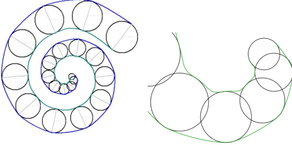
In the following, 2D ball skinning algorithms will be covered. Let’s take a series of circles. Slabaugh introduced an energy function for making a skinning curve (see Figure 1).
Figure 1: Slabaugh’s skinning curves for the series of circles and the zoomed wavy inner part
If the inner part is enlarged, it can be noticed that the inner curve is very wavy.
If we take the same enlarged inner part of the Kunkli-Hoffmann’s algorithm, it can be noticed that the inner curve is following only one direction (see Figure 2). There are no inflection points.
It seems that the number of the inflection points of a curve is a good measure for the visual smoothness.
Figure 2: The result of the Kunkli-Hoffmann interpolation curve
2. Measurement for Visual Smoothness
Let’s introduce a measure that will sum the inflection points of the Bézier curve parts that make up the whole curve.
“The algebraic form of a parametric cubic belongs to one of three projective types, as shown in Figure 4. Any arbitrary cubic curve can be classified as a serpentine, cusp, or loop. A very old result (Salmon 1852) on cubic curves states that all three types of cubic curves will have an algebraic representation that can be writtenk3−lmn= 0, wherek,l,m, andnare linear functionals corresponding to linesk,l,m, andnas in Figure 3.
k
l n m
l n m
k
l m n
k
a) b) c)
Figure 3: All parametric cubic plane curves can be classified as the parameterization of some segment of one of these three curve types.
a) Serpentine curve. This curve has three collinear inflection points (on linek) with tangent linesl,mandnat those inflections.
b) Loop curve. This curve has one inflection and one double point withkthe line through them. The lineslandmare the tangents to the curve at the double point andnis the tangent at the inflection.
c) Cusp curve. This curve has one inflection point and one cusp, withk the line through them. The linel=mis the tangent at the
cusp andnis the tangent at the inflection. [4]
A cubic Bézier curve in homogeneous parametric form is written
C(s, t) = [(s−t)3 3(s−t)2s 3(s−t)2s2 s3]·
b0
b1
b2
b3
,
where thebi are cubic Bézier control points.
The first step is to compute the coefficients of the function I(s, t) whose roots correspond to inflection points of C(s, t). An inflection point is where the curve changes its bending direction, defined mathematically as parameter values where the first and second derivatives of C(s, t) are linearly dependent. The derivation of the functionIis not needed for the current purposes. For integral cubic curves,
I(s, t) =t(3d1s2−3d2st+d3t2),
where
d1=a1−2a2+ 3a3, d2=−a2+ 3a3, d3= 3a3
and
a1=b0·(b3×b2), a2=b1·(b0×b3), a3=b2·(b1×b1).
The functionIis a cubic with three roots, not all necessarily real. It is the number of distinct real roots of I(s, t) that determines the type of the cubic curve. For integral cubic curves, [s t] = [1 0]is always a root ofI(s, t). This means that the remaining roots ofI(s, t)can be found using the quadratic formula, rather than by the more general solution of a cubic – a significant simplification over the general rational curve algorithm.
The cubic curve classification reduces to knowing the sign of the discriminant ofI(s, t), defined as
discr(I) =d21(3d22−4d1d3).
Ifdiscr(I)is positive, the curve is a serpentine; if negative, it is a loop; and if zero, a cusp. Although it is true that all cubic curves are one of these three types, not all configurations of four Bézier control points result in cubic curves. It is possible to represent quadratic curves, lines, or even single points in cubic Bézier form. The procedure will detect these cases, and the rendering algorithm can handle them. It is not needed to consider (or render) lines or points, because the convex hull of the Bézier control points in these cases has zero area and, therefore, no pixel coverage.
The general classification of cubic Bézier curves is given by Table 1.
Serpentine discr(I)>0
Cusp discr(I) = 0
Loop discr(I)<0 Quadratic d1=d2= 0 Line d1=d2=d3= 0 Point b0=b1=b2=b3
Table 1: Cubic Curve Classification
If the Bézier control points have exact floating-point coordinates, the classifica- tion given in Table 1 can be done exactly. That is, there is no ambiguity between cases, because discr(I) and all intermediate variables can be derived from exact floating representations.” [5]
A serpentine has three inflection points while a cusp have one inflection point.
Bézier curves of other type will have one inflection point if b0 andb3 are on the
two different sides of the line defined byb1andb2. It can be easily determined by the scalar product of the homogeneous coordinates of the control points and the equation of the line.
To define an exact measurement for visual smoothness, the number of these inflection points shall be summarized. This measurement shall be extended by the inflection points at the joining points of the Bézier curves that make up the interpolating curves used for skinning the series of circles.
Two joining Bézier curves defined by (b0,b1,b2,b3) and (b3,b4,b5,b6) will have an inflection point in the joining b3 control point if b1 and b5 are on the different sides of the line defined byb2,b3 andb4 control points.
The final measurement will be the summarized inflection points inside the Bézier curves and the inflection points at the joining end points of the curves.
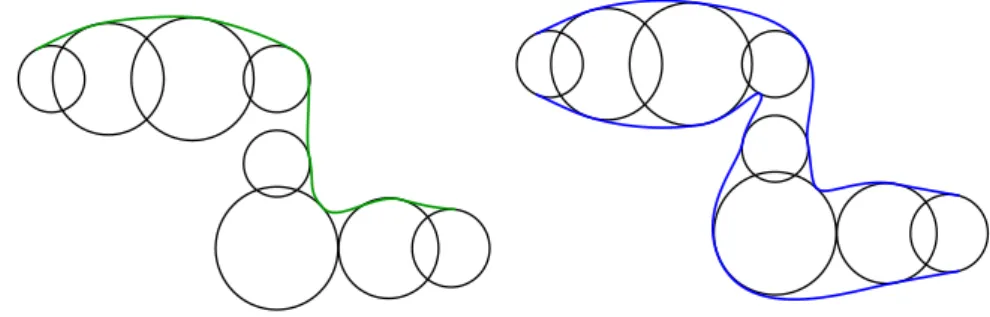
Figure 4 shows that Slabaugh’s algorithm has five, while the Kunkli-Hoffmann’s curve has only four inflection points on the top skinning curves.
Figure 4: Second example for Slabaugh and Kunkli-Hoffmann curves for the same series of circles
3. Results
Examining the interpolating inner curves only of the last six inner circles of the series of Figure 1 and Figure 2 shows that Slabaugh’s curve has five inflection point among the six circles while Kunkli-Hoffmann’s curve has none. Even on the more complex Figure 4 this ratio is five to four. Thus, in both cases the second curve is more smooth.
Testing for further arrangements, Kunkli-Hoffmann’s interpolation curves usu- ally have fewer inflection points and this way they yield a more smooth interpo- lating curve. By using these more smooth curves and surfaces, better customized sulutions can be provided for simulations or avatars’ heads and bodies.
References
[1] G. Slabaugh, G. Unal, T. Fang, J. Rossignac, B. Whited,Variational skinning of an ordered set of discrete 2D balls,Lecture Notes on Computer Science,Vol. 4795 (2008), 450–461.
[2] R. Kunkli,Localization of touching points for interpolation of discrete circles,An- nales Mathematicae et Informaticae, 36 (2009), 103–110.
[3] R. Kunkli, M. Hoffmann,Skinning of circles and spheres, Computer Aided Geo- metric Design, 27 (2010), 611–621.
[4] C. Loop, J. Blinn, Resolution independent curve rendering using programmable graphics hardware, ACM Transactions on Graphics (TOG) - Proceedings of ACM SIGGRAPH 2005, Vol. 24 Issue 3 (July 2005), 1000–1009.
[5] H. Nguyen,GPU Gems 3 (Chapter 25. Rendering Vector Art on the GPU),Addison- Wesley Professional, (2007), 543–562.