On geometric Hermite arcs ∗
Imre Juhász
Department of Descriptive Geometry, University of Miskolc, Hungary agtji@uni-miskolc.hu
Submitted June 3, 2015 — Accepted September 27, 2015
Abstract
A geometric Hermite arc is a cubic curve in the plane that is specified by its endpoints along with unit tangent vectors and signed curvatures at them. This problem has already been solved by means of numerical proce- dures. Based on projective geometric considerations, we deduce the problem to finding the base points of a pencil of conics, that reduces the original quartic problem to a cubic one that easier can exactly be solved. A simple solvability criterion is also provided.
Keywords:Hermite arc, geometric constraint, pencil of conincs MSC:65D17, 68U07
1. Introduction
In Computer Aided Geometric Design curves are often specified by means of some constraints that the required curve has to fulfill, instead of by those data that are necessary for a certain representation form (e.g. Bézier or B-spline). A classical example is the Hermite arc, where endpoints are given along with the tangent vector (i.e. the first derivative of the curve with respect to the parameter) at them from which data a cubic arc has to be determined. This task always has a unique solution.
A slight modification of the previous problem is the so called geometric Hermite arc, where endpoints of a cubic arc in plane with unit tangent vectors and signed
∗This research was carried out in the framework of the Center of Excellence of Mechatronics and Logistics at the University of Miskolc.
http://ami.ektf.hu
61
curvatures at them are given. Unlike in the classical Hermite arc, a solution to this problem does not always exist.
This problem pops up in [1] in connection with equidistants of plane cubic spline curves. In [2]G2 cubic plane interpolating splines are constructed with geometric Hermite arcs, moreover a thorough analysis and a criterion for solvability is pro- vided. In [3] G2 end conditions are discussed for C2 planar cubic interpolating splines (Ferguson splines). [4] studies transition curves between circular and conic arcs meeting G2 continuity requirements, while [5] provides G2 transition curves between two circles. There are several generalizations of the problem. [6] gener- alizes the problem to rational cubics and [7] to interpolating spline surfaces, while [8] restricts the solution to Pythagorean-hodograph cubics.
No matter in what way we seek the solution to the original problem, it always ends in a system of quadratic equations in two variables. In all the cited publica- tions this system is solved numerically. Equations of the system are quite special that gives the hope of a simple exact solution. In this contribution we provide such a solution based on projective geometric considerations.
2. Bézier points of the arc
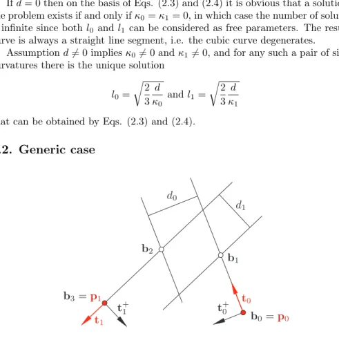
Let us denote the endpoints by p0 and p1, the signed curvatures at them by κ0
andκ1, and the unit tangent vectors byt0 andt1.We want to produce the Bézier representation
b(u) = X3 i=0
Bi3(u)bi, u∈[0,1]
of the cubic Hermite arc, whereBi3(u)denotes theith cubic Bernstein polynomial.
Its control points {bi}3i=0 can be expressed in the form b0=p0,
b3=p1,
b1=p0+l0t0, (2.1)
b2=p1−l1t1, (2.2)
in which positive lengthsl0 andl1 are unknown.
The signed curvature of a cubic planar Bézier curve is of the form κ(u) = ˙b(u)∧b¨(u)
˙b(u)3
,
where ˙b(u)∧¨b(u)is the third component of the cross product of the vectors ˙b(u) andb¨(u). Its value at the first and last points are
κ0:=κ(0) =2 (b1−b0)∧(b2−b1) 3l30
=2A(b0,b1,b2) 3l03 and
κ1:=κ(1) =2 (b2−b1)∧(b3−b2) 3l31
=2A(b1,b2,b3) 3l13
respectively, whereA(a,b,c)stands for the signed area of the triangle determined by the sequence of vertices a,b,c. Denoting the signed distance of the control pointb2 from the directed straight lineb0,b1 byd0(cf. Fig. 1) we obtain for the signed area
A(b0,b1,b2) =l0d0
and for the signed curvature 2
κ0=2 3
d0
l02. (2.3)
Analogously, the signed curvature κ1 is of the form κ1=2
3 d1
l12, (2.4)
whered1is the signed distance of the control pointb1from the directed lineb2,b3.
Figure 1: The signed curvature at the first point of a Bézier curve is proportional to the signed area of the triangle with ver-
ticesb0,b1,b2
2.1. Parallel tangent vectors
If t0kt1 then Eqs. (2.1) and (2.2) imply equality d=|d0| =|d1|, whered is the distance between the parallel lines determined by point and direction vector pairs p0,t0 andp1,t1.
Ifd= 0then on the basis of Eqs. (2.3) and (2.4) it is obvious that a solution to the problem exists if and only ifκ0=κ1= 0, in which case the number of solutions is infinite since both l0 andl1 can be considered as free parameters. The resulted curve is always a straight line segment, i.e. the cubic curve degenerates.
Assumptiond6= 0impliesκ06= 0andκ16= 0, and for any such a pair of signed curvatures there is the unique solution
l0= r2
3 d
κ0 andl1= r2
3 d κ1
that can be obtained by Eqs. (2.3) and (2.4).
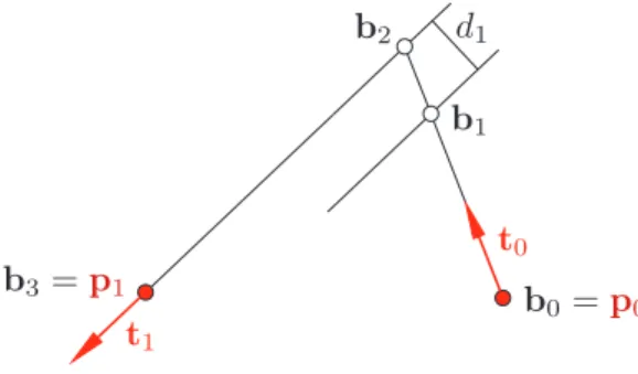
2.2. Generic case
Figure 2: Determination of Bézier points
Hereafter we assume thatt0∦t1. Using the notations of Fig. 2, distance d1 is of the form
d1= (b1−b3)·t+1 = (p0+l0t0−p1)·t+1
=l0t0·t+1 −(p1−p0)·t+1 and the distanced0 is
d0= (b2−b0)·t+0 = (p1−l1t1−p0)·t+0
= (p1−p0)·t+0 −l1t1·t+0.
Introducing notationsa=t0·t+1 =−t1·t+0,b= (p1−p0)·t+1 andc= (p1−p0)·t+0, wheret+i denotes the positive normal vector ofti, i.e. ti is rotated throughπ/2in counterclockwise direction, we obtain equalities
d0=al1+c, (2.5)
d1=al0−b. (2.6) Eqs. (2.3) and (2.5) yield equation
3κ0l02−2al1−2c= 0 (2.7)
and Eqs. (2.4) and (2.6)
3κ1l12−2al0+ 2b= 0 (2.8)
for the unknown distancesl0 andl1. Therefore, the solution of the geometric Her- mite interpolation is reduced to the solution of the system of quadratic equations (2.7), (2.8) of unknownsl0and l1. This system does not always has a solution, or if it has, the the obtained values ofl0and l1 are not necessarily positive.
Before we solve the generic case, we have a look at those special cases when one or both of the curvatures vanish. If, e.g. κ0 = 0 and κ1 6= 0 then the problem is reduced to a linear one, the solution is
l0=3 2κ1
c2 a3 +b
a, l1=−c
a
and control points b0,b1 and b2 become collinear, since κ0 = 0 implies d0 = 0.
This case is illustrated in Fig. 3.
Figure 3: The caseκ0= 0andκ16= 0
If both curvatures vanish, thenκ0=κ1= 0 involvesd0=d1 = 0thus control pointsb1andb2 coincide and are the point of intersection of the two tangent lines that must exist due to the assumption t0∦t1 (cf. Fig. 4).
3. An exact solution of the quadratic system
Hereafter we assume thatt0∦t1 andκ06= 0,κ16= 0. In this case equalities (2.7) and (2.8) describe parabolas in the coordinate system(l0, l1)the axis of which are
Figure 4: The caseκ0=κ1= 0
perpendicular. Using homogeneous coordinates, the matrices of these parabolas are
A=
0 0 −a 0 3κ1 0
−a 0 2b
andB=
3κ0 0 0
0 0 −a
0 −a −2c
.
To solve the system means to find points of intersection of these parabolas. These two parabolas establish a pencil of conics, the elements of which are of the form
C=αA+βB, α, β∈R, |α|+|β| 6= 0. (3.1) To find points of intersection of the parabolas is equivalent to determine the base points of the pencil. One of the parameters can be eliminated from matrix (3.1), since matricesCandγC,(06=γ∈R)determine the same conic, therefore we will study the matrix
C(λ) =λA+B
=
3κ0 0 −λa 0 3λκ1 −a
−λa −a 2 (λb−c)
,λ∈R. (3.2)
If we can find a degenerate element of this pencil, i.e. an element that is composed of a pair of straight lines, then we can reduce the original quartic problem to a quadratic one. The degenerate element of the pencil is provided by such a λ for whichdet (C(λ)) = 0, that yields the cubic polynomial
κ1a2λ3−6bκ0κ1λ2+ 6cκ0κ1λ+κ0a2= 0.
One real root of this cubic polynomial has to be determined, that always exists.
After all, the quartic problem can only be reduced to a cubic one using this method, however this can exactly be solved in a simple way without a numerical procedure.
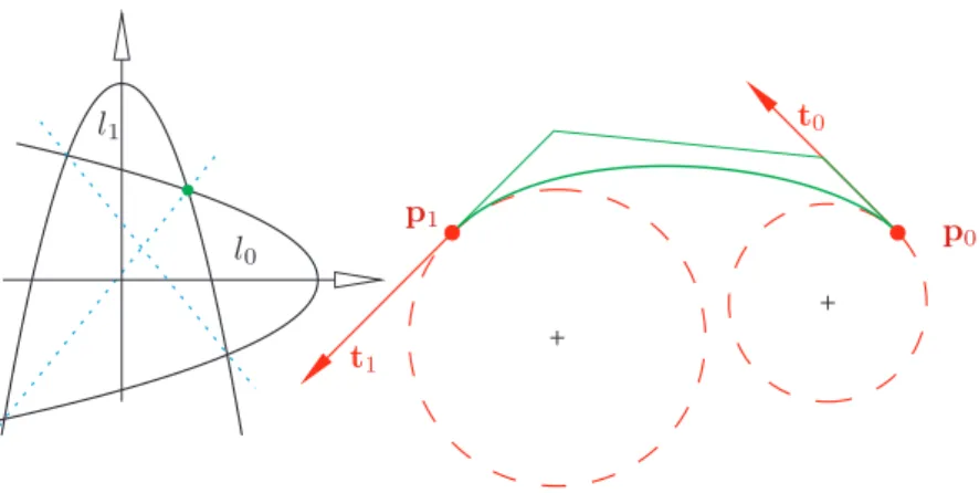
Parabolas (2.7) and (2.8) are of special position, their axes are perpendicular, and the pencil determined by them always contains an element which is a circle.
Indeed, it is easy to check that absolute (or imaginary) circle points (points at which the line at infinity intersects any circle)
1 i 0 T and
−1 i 0 T
Figure 5: One positive solution (right) along with the correspond- ing pair of parabolas and a degenerated element (blue dotted) of the pencil determined by them (left). Settings are p0 = [2 0]T, p1= [−1 0]T,t0= [−1 1]T,t1= [−1 −1]T,κ0= 1.5,κ1= 1(For interpretation of the references to color in this figure legend, the
reader is referred to the pdf version of this article.)
are on the element of the pencil (3.2) that corresponds to λ= κ0
κ1,
providedκ16= 0, that we have already excluded. The matrix of this circle is
3κ0 0 −κκ01a
0 3κ0 −a
−κκ01a −a 2
κ0
κ1b−c
,
therefore the square of its radius is r2= 2
3κ0
c−κ0
κ1
b
. (3.3)
If (3.3) is positive (note that the circle can be imaginary as well) then parabolas (2.7) and (2.8) have real points on common, i.e. the system of quadratic equations has a solution. Note, that this is a criterion just for the solvability of the system and not for the positive solution.
In practice, positive solutions (bothl0 andl1 are positive) are used in general, since only in this case will the direction of tangent vectors be kept. In the coordinate system(l0, l1) the axis of parabolas (2.7) and (2.8) coincide with the axes l0 and l1of the coordinate system, respectively, thus the number of positive solutions can be 0,1,2or 3.
As it is specified in [2], in the generic case there can be a positive solution if products
t0∧t1, (p1−p0)∧t1, t0∧(p1−p0)
have the same sign that coincides with the sing of κ0 and κ1. In this case the existence of a positive solution can be guaranteed by adjusting the magnitude of curvatures, i.e. curvatures can be used as shape parameters. Fig. 5 illustrates a case of one positive solution.
References
[1] Klass, R. An offset spline approximation for plane cubic splines, Computer–Aided Design, Vol. 15 (1983), No. 5, 297–299.
[2] de Boor, C., Hölling, K., Sabin, M. High accuracy geometric Hermite interpo- lation,Computer Aided Geometric Design, Vol. 4 (1987), No. 4, 269–278.
[3] Ginnis, A.I., Kaklis, P.D. Planar C2 cubic spline interpolation under geometric boundary conditions,Computer Aided Geometric Design, Vol. 19 (2002), No. 5, 345–
363.
[4] Meek, D.S., Walton D.J. Planar G2 Hermite interpolation with some fair, C- shaped curves,Journal of Computational and Applied Mathematics, Vol. 139 (2002), No. 1, 141–161.
[5] Habib, Z., Sakai, M.G2 cubic transition between two circles with shape control, Journal of Computational and Applied Mathematics, Vol. 223 (2009), No. 1, 133–144.
[6] Sakai, M. Osculatory interpolation, Computer Aided Geometric Design, Vol. 18 (2001), No. 8, 739–750.
[7] Valasek, G., Vida, J. C2 Geometric Spline Surfaces, Proceedings of the Seventh Hungarian Conference on Computer Graphics and Geometry, (2014), 7–12.
[8] Jaklič, G., Kozak, J., Krajnc, M., Vitrih, V., Žagar, E.On interpolation by planar cubicG2Pythagorean-hodograph spline curves,Mathematics of Computation, Vol. 79 (2010), No. 269, 305–326.