Fracture network characterization using 1D and 2D data of the Mórágy Granite body, southern Hungary
Tivadar M. Tóth
PII: S0191-8141(18)30284-0 DOI: 10.1016/j.jsg.2018.05.029 Reference: SG 3670
To appear in: Journal of Structural Geology Received Date: 18 December 2017
Revised Date: 23 May 2018 Accepted Date: 29 May 2018
Please cite this article as: M. Tóth, T., Fracture network characterization using 1D and 2D data of the Mórágy Granite body, southern Hungary, Journal of Structural Geology (2018), doi: 10.1016/
j.jsg.2018.05.029.
This is a PDF file of an unedited manuscript that has been accepted for publication. As a service to our customers we are providing this early version of the manuscript. The manuscript will undergo copyediting, typesetting, and review of the resulting proof before it is published in its final form. Please note that during the production process errors may be discovered which could affect the content, and all legal disclaimers that apply to the journal pertain.
M AN US CR IP T
AC CE PT ED
F
RACTURE NETWORK CHARACTERIZATION USING1D
AND2D
DATA OF THE 1M
ÓRÁGYG
RANITE BODY, S
OUTHERNH
UNGARY 23
M. Tóth, Tivadar 4
University of Szeged, Department of Mineralogy, Geochemistry and Petrology, 5
mtoth@geo.u-szeged.hu 6
7 8
ABSTRACT
9
A disposal system for low- and medium-level nuclear waste in Hungary is being constructed 10
inside the fractured rock body of the Lower Carboniferous Mórágy Granite. Previous studies 11
proved that the granitoid massif is rather heterogeneous in terms of lithological composition, 12
brittle structure and hydrodynamic behaviour. A significant part of the body consists of 13
monzogranite, while other portions are more mafic in composition and are monzonites. As a 14
result of at least three significant brittle deformation events, the area is at present crosscut by 15
wide shear zones that separate intensively fractured zones and poorly deformed domains 16
among them. Due to late mineralization processes, some of these fractured zones are totally 17
sealed and cannot conduct fluids, while others are excellent migration pathways. The spatial 18
distribution of these two types nevertheless does not show any systematics. Hydrodynamic 19
behaviour clearly reflects this heterogeneous picture; in some places, hydraulic jumps as great 20
as 25 m at compartment boundaries can be detected.
21
In this study, the fracture network of the Mórágy Granite body is evaluated from a geometric 22
aspect using datasets measured at a wide range of scales. 2D digitized images of a hand 23
specimen, one large (20 × 60 m) and 12 smaller subvertical wall rocks (outcrops) and 120 24
images from tunnel faces representing the ground level of the underground repository site 25
were analysed. Moreover, 1D data from 13 wells that all penetrate the granitoid massif were 26
studied. Based on measured geometric data (spatial position, length, orientation, and aperture) 27
fracture networks are simulated to study connectivity relations and for computing the 28
fractured porosity and permeability at different scales. The results prove the scale-invariant 29
geometry of the fracture system. Geostatistical calculations indicate that measurable fracture 30
geometry parameters behave as regionalized variables and so can be extended spatially.
31
Estimated localities of connected subsystems fit very well with fault zones mapped 32
M AN US CR IP T
AC CE PT ED
previously. Moreover, the spatial position of regimes of different hydrodynamic behaviours 33
can be explained by connectivity relations both regionally and within wells.
34 35 36
INTRODUCTION
37
A disposal system for Hungary's low- and medium-level nuclear waste is being constructed 38
inside the fractured rock body of the Lower Carboniferous Mórágy Granite. There are only a 39
few outcrops available for studying the rock on the surface; the granite body is essentially 40
covered by younger Pliocene and Pleistocene sediments. As rock heterogeneity relations as 41
well as large-scale structures of the area can hardly be examined by traditional outcrop survey 42
or using remote-sensing approaches, numerous wells penetrating the granite body reveal the 43
petrological and structural circumstances. Moreover, two access tunnels were excavated 44
underground.
45
Fracture systems play an essential role in fluid flow and transport processes in hard rock 46
bodies. Over the last few decades (e.g., Maros et al., 2004, 2010), a detailed structural 47
geological evaluation of the faults and fault systems in the Mórágy Granite has been 48
completed; the most important deformation zones are well-known and have been published on 49
high-resolution maps. Nevertheless, fracture networks at micro- and meso-scales, which play 50
a significant role in hydrodynamic behaviour of the hard rock body (Anders et al., 2014), are 51
basically unknown and are studied in the framework of the present project. The most essential 52
questions are whether the single fractures form a communicating network or not, how large 53
the communicating subsystems are and where they are located. To answer these questions, 54
fracture networks are simulated based on measurable geometric parameters. Fracture 55
networks are usually handled as scale invariant geometrical objects (e.g., Korvin, 1992, 56
Turcotte, 1992, Long, 1996, Weiss, 2001). To test whether the fracture network of the 57
Mórágy Granite can be examined by the corresponding methodology, fracture systems at a 58
wide spectrum of scales (surface outcrop, tunnel faces, borehole and hand specimen data) are 59
evaluated simultaneously using the same set of methods. That is, data used for simulation 60
work are received by a combined analysis of 1D and 2D fracture patterns. Modelling requires 61
geometric data regarding fracture size distribution, spatial density and orientation. Simulated 62
models are afterwards available to understand features of the fractured rock body concerning 63
hydrodynamic behaviour, such as connectivity, porosity and permeability.
64 65 66
M AN US CR IP T
AC CE PT ED
GEOLOGICAL BACKGROUND
67
The Bátaapáti Site is located in the southern part of Hungary (fig. 1); the Carboniferous 68
Mórágy Granite Formation (MGF) was selected as the repository of low- and intermediate- 69
level radioactive wastes. Petrographically the MGF was described by Király and Koroknai 70
(2004) as a porphyritic monzogranite intercalated with a more mafic variety of monzonitic 71
composition without a sharp contact (fig. 2). According to the recent models the combination 72
of the two granitoid rock types developed through a magma-mixing process. The whole rock 73
body is also crosscut by swarms of aplitic dykes of various widths. Two major deformation 74
events developed the ductile structure of the MGF (Király, Koroknai, 2004). The magma- 75
mixing process coincided with formation of a generally NE-SW striking igneous foliation 76
mostly with a steep NW dip. During the next phase, deformation resulted in steeply foliated 77
mylonitic zones, basically with a NE-SW strike again. The upper several tens of metres of the 78
granitoid body are strongly altered and weathered and are covered by Miocene, Pliocene and 79
Quaternary sediments with a thickness of approximately 50 m on the hilltops and thinning 80
towards the valleys. As a consequence, only a few surface outcrops exist that are available for 81
petrological and structural study. Many details of mineralogical, geochemical and petrological 82
circumstances of the MGF, not directly concerning the present project, are presented in Király 83
(2010) and references therein.
84
The brittle deformation history of the area and the mechanisms of different structural 85
events are discussed in detail by Maros et al. (2004). Most structures exhibit two typical 86
orientations: NE-SW (the dominant set) and perpendicular to this (NW-SE) (fig. 1). Small- 87
scale fracture orientations are very similar to those appearing at large-scale zones (Benedek 88
and Molnár, 2013). When studying fracture networks from a geometric aspect, fracture size 89
appears to be related to the distance from major fault zones; larger fractures appear to cluster 90
preferentially around them (Benedek and Molnár, 2013). Nevertheless, length exponents were 91
found varying within a very narrow range (2.15–2.44) at different scales (outcrop scale: 0.4–7 92
m trace length, vertical seismic profile measurements: 6–40 m trace length, seismic line 93
measurements: 100–400 m trace length, Benedek and Dankó, 2009).
94
Generally, a fractured reservoir system can be divided into two subsystems; more 95
permeable discontinuities surround a less permeable matrix (Neuman, 2005). This theoretical 96
model is the basis of the hydrostructural concept of the MGF as well (Molnár et al., 2010).
97
Benedek and Molnár (2013) distinguish two hydraulic domains inside the fractured granitoid 98
body; less transmissive blocks and more transmissive zones (LTBs and MTZs, respectively).
99
Nevertheless, the definition of the boundaries between these two domains is highly subjective.
100
M AN US CR IP T
AC CE PT ED
The MTZs follow both NE-SW and NW-SE directions, with the most significant flows 101
observed along the NE-SW zones. Fractures inside an LTB, on the other hand, cannot be 102
represented by any single characteristic orientation. Although hydraulically active fracture 103
zones are frequent in the study area, fracture clusters are not entirely interconnected. As a 104
consequence, there is no hydraulic connectivity between all points of the studied region 105
(Benedek and Dankó, 2009). According to Benedek et al. (2009) such a compartmentalization 106
is not exclusively the result of fracture geometry, but in part the consequence of intensive 107
secondary mineralization of certain fracture zones. At a site scale, the resulting strongly 108
compartmentalized character of the fracture system causes the high complexity of the flow 109
pattern as well. Neighbouring compartments usually have slightly different heads (1–5 m), 110
while hydraulic jumps at compartment boundaries defined by sealed faults may be as great as 111
5–25 m. In general, hydrodynamic behaviour and especially the calculated transmissivity is 112
significantly different for the two differently deformed regions, varying being 10-12 and 10-6 113
m2/s for the fresh granite of the LTBs and 8*10-6 and 2*10-5 m2/s for the MTZs (Balla et al.
114
2004, Rotár-Szalkai et al, 2006).
115 116 117
SAMPLES
118
In this study of the brittle structures of the Mórágy granite body, 1D and 2D information 119
collected from diverse localities and scales were evaluated. The most detailed 2D fracture 120
network dataset is represented by a subvertical outcrop, 20 × 60 m in size, at the SW part of 121
the study area. From the same outcrop, a hand specimen (20 × 30 cm in size) was investigated 122
as well. In addition to the hand specimen and the whole wall, 12 smaller, equally sized 123
rectangular portions of the wall have been documented and evaluated.
124
Additional 2D fracture network data were derived from tunnel faces representing the 125
ground level of the underground repository site (fig. 1, inset). Altogether 120 JointMetriX3D 126
(Gaich et al., 2005, Deák and Molnos, 2007) images were handled with an equal 20 m lag 127
between the neighbouring sampling points. At least 300 single fractures were digitized and 128
evaluated in each JointMetriX3D image.
129
The series of intersection points between the fracture system in the real 3D and a line 130
(usually a borehole) defines a 1D data set. 1D fracture data were obtained by evaluating well- 131
logs (BHTV, acoustic borehole televiewer; Zilahi-Sebess et al. 2003) and core scanner (CS, 132
Maros and Palotás, 2000) images from 14 wells, representing the whole study area (fig. 2).
133 134
M AN US CR IP T
AC CE PT ED
135
METHODS
136
Fracture networks can be characterized from numerous structural geological points of view 137
and by diverse measurable geometric parameters. In the latter approach, each single fracture 138
must be represented by an appropriate geometric shape. In most approximations a polygon or 139
a circle is used for this reason (Neuman, 2005). Hereafter, this last approach is followed, and 140
so the most important geometric parameters to define a fracture are length (diameter), spatial 141
position of the centre and orientation. To calculate porosity and permeability data for the 142
fracture network, the fractures must have positive volume, so instead of pure circles, each 143
fracture is represented by a flat cylinder geometrically (parallel plate model, Witherspoon et 144
al., 1980; Neuzil, Tracy, 1981; Zimmerman, Bodvarsson, 1996). Furthermore, in order to 145
understand spatial behaviour of fracture networks, a large set of discrete fractures should be 146
studied simultaneously, and distributions of length, aperture, orientation (strike and dip) and 147
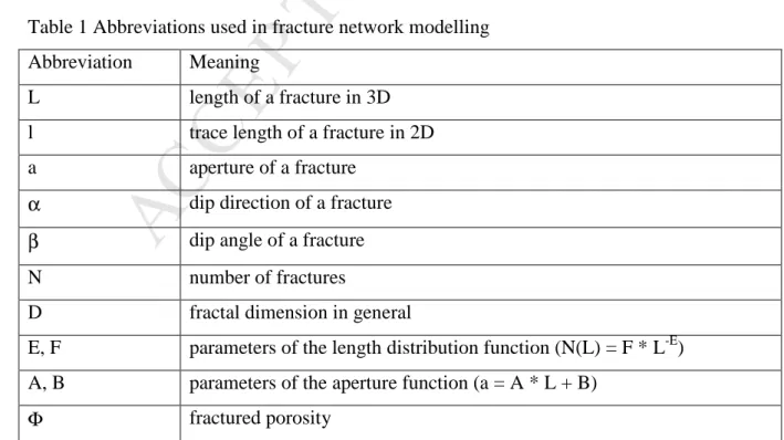
spatial density of fracture midpoints are used. Abbreviations of the geometric parameters 148
applied are summarized in Table 1.
149
During the fracture network modelling process three sets of methods are used. 1) The 150
first of them deals with determination of fracture network geometric parameters. 2) Prior to 151
fracture network simulation using the above parameters, they should be interpolated for the 152
studied area. 3) Finally, appropriate simulation software should be applied for 3D fracture 153
network modelling.
154 155
Geometric parameters of fractures 156
Length distribution 157
Both concerning conductivity and fluid storage, length distribution is an essential parameter 158
of fracture networks. According to numerous previous studies, fracture lengths follow a 159
power law distribution (Yielding et al., 1992, Min et al., 2004), that is N(L) = F * L-E. Using 160
an appropriate number of single fractures (at least 300), on any 2D surface, the two 161
parameters E (the length exponent) and F can be determined by image-analysis methods on 162
digital photos (Healy et al., 2017). First, the frequency distribution function of fracture trace 163
lengths measured on any photo were plotted. When computing the histogram, the number of 164
classes (k) was determined so that k = 2 * INT(log2(N(L)). Length exponent is afterwards the 165
slope of the best fit line on the Log(L)-log(N(L)) plot. Because of representativity defects, the 166
smallest and longest fractures usually do not fit to this line and so must be left out of the 167
analysis. This approach was followed when evaluating data of the outcrop, the hand specimen 168
M AN US CR IP T
AC CE PT ED
and the tunnel faces (fig. 3). Instead of using the histogram on doubly logarithmic axes, to 169
find the best fit line Rizzo et al. (2017) suggest to apply maximum likelihood estimator.
170
To determine the length exponent in the case of 1D data sets, the same equation (N(L) 171
= F * L-E) can be utilized as previously presented. The mathematical background of how to 172
obtain the E parameter using 1D point series is too long to recall here; it is described in detail 173
in M. Tóth (2010). Using this approach, a unique E parameter has been determined for each 174
studied well (fig. 2).
175 176
Spatial density of fracture midpoints 177
Numerous previous studies proved that fracture systems behave geometrically in a fractal-like 178
pattern (Barton and Larsen, 1985, La Pointe, 1988, Hirata, 1989, Matsumoto et al., 1992, 179
Kranz, 1994, Tsuchiya and Nakatsuka, 1995, Roberts et al., 1998, among others).
180
Consequently, the spatial distribution of single fractures can be characterized by the fractal 181
dimension of the fracture midpoints. Fractal dimension is computed using the box-counting 182
method, applied to fracture network analysis by numerous authors previously (Mandelbrot, 183
1983, Mandelbrot, 1985, Barton and Larsen, 1985, Barton, 1995). Here, a non-overlapping 184
regular grid of square boxes was used during the box-counting analysis. In the algorithm, the 185
number of boxes (N(r)) required to cover the pattern of fracture seeds is counted. Fractal 186
dimension is calculated by computing how this number changes in making the grid finer, 187
afterwards: N(r) ~ r-D (fig. 3). For box-counting calculations, the BENOIT 1.0 software was 188
used Benoit 1.0 (Trusoft, 1997).
189
To determine fractal dimension in the case of 1D scanlines, a fractional Brownian 190
motion analysis was followed as described in detail in M. Tóth (2010). As R/S (Rescaled 191
Range) analysis applied in determining fractal dimension along a scanline needs at least 400 192
points (single fractures) to reach reasonably low uncertainty (Katsev and L’Heureux,2003), D 193
parameters were calculated every 25 m as a minimum. Within this depth interval each well 194
crosscuts the desired number of fractures, making D logging along the wells possible.
195 196
Fracture aperture 197
Most previous studies (de Dreuzy et al., 2002, Ortega et al., 2006) confirm that, similar to 198
length, aperture data follow a power law distribution. Nevertheless, the two parameters are 199
not independent of each other; instead, a tight linear relationship is also suggested between 200
them such that: a = A * L + B (Pollard and Segall, 1987, Gudmundsson et al., 2001). Both 201
measurements on naturally fractured rock bodies and theoretical deliberation confirm that a/L 202
M AN US CR IP T
AC CE PT ED
typically varies by an order of magnitude of 10-2 to 10-3 for most rock types (Opheim and 203
Gudmundsson, 1989, Vermilye and Scholz, 1995). In the studied case, the aperture was 204
measured exclusively on the hand specimen under a binocular microscope (50×
205
magnification). For each microfracture, aperture was determined at a minimum of 3 points.
206 207
Fracture orientation 208
In the near-well fracture network modelling procedure, orientation data (dip direction and dip 209
angle) of individual fractures obtained by BHTV interpretation were used (Szongoth et al., 210
2004). For modelling the underground site, orientation data measured in the closest well (Üh- 211
2) were used.
212 213
Interpolation of the fracture network parameters 214
The D values were computed for each well for every 25-m interval making generation of a 215
series of horizontal D-maps possible. Nevertheless, the reduced number of wells deemed 216
reliable for mapping did not allow application of sophisticated geostatistical methods 217
(semivariogram analysis and interpolation using kriging). Therefore, for interpolation and 218
extrapolation, the minimal curvature method (Dietze, Schmidt, 1988 and references therein) 219
was chosen in a grid net of 100 × 100 × 25 m sized cells. In the case of the underground 220
repository site, georeferenced photos are available for precise calculations. To understand the 221
spatial variability of fracture parameters, semivariogram and variogram surfaces were 222
computed using the Variowin 2.2 software (Pannatier, 1996). Considering the variogram data, 223
ordinary kriging was applied for parameter interpolation. During the procedure, 30 × 30 × 30 224
m sized cells were used.
225
In both studied cases (whole area and underground site), the interpolated fracture 226
parameters served as input data for the fracture network modelling procedure.
227 228
Fracture network modelling 229
During a previous modelling study in a small subarea of the recent study area, Benedek and 230
Molnár (2013) used the Poisson point process as a spatial model for fracture localization. In 231
that model, fractures represent a random function in space. Hereafter, for simulating fracture 232
networks in 3D, the RepSim code was used (M. Tóth, 2010, M. Tóth and Vass, 2011, Bauer 233
and M. Tóth, 2016). In this DFN (discrete fracture network) software penny-shaped single 234
fractures are generated in a stochastic manner with a given parameter set of (D, E, F, α, β) 235
measured in the real fractured rock body. Thanks to the stochastic approach in the fracture 236
M AN US CR IP T
AC CE PT ED
system generation, numerous equally probable networks can be simulated and evaluated.
237
Aperture is calculated for each discrete fracture in a deterministic manner assuming the 238
aforementioned length-aperture relationship (Odling, 1993). One of the most essential 239
features of a simulated fracture network is the size and spatial position of its communicating 240
subsystems. In the applied software, they can be found using a properly optimized trial-and- 241
error algorithm (M. Tóth and Vass, 2011).
242
Fractured porosity can be defined as 243
244
V
=Vf Φ
. (1)
245 246
In the case of cubic cells V=r3, the total volume of the fractures inside a certain cube (Vf) 247
can be approximated well by the lower Riemann sum, that is, 248
249
∑∑
=
⋅
= n ⋅
1
i j
ij ij
n r a Vf l
, (2)
250 251
and the porosity is in the form of 252
253
∑∑
=
⋅
=
Φ n
1
i j
ij
2 lij a
r
* n
1
(3) 254
255
The permeability of a fractured rock mass can be represented by a 3×3 permeability 256
tensor. In the RepSim code, it is calculated using the slightly modified algorithm of Oda 257
(1985). Thus, under Darcy’s law, 258
259
i j i
i g k J
v = ⋅ρ⋅ , ⋅
µ (4)
260 261
where v is the specific flow rate, µ is the dynamic viscosity, ρ is the density of the fluid, and J 262
is the hydraulic gradient. On the other hand, as fluid can percolate only along fractures, over a 263
given volume, 264
265
M AN US CR IP T
AC CE PT ED
∫
⋅⋅
= if f
i v dV
v V1
(5) 266
267
where vf is the flow velocity in a discrete fracture. This is approximated ad libitum by 268
269
∑
⋅⋅
=
f
f if
i v V
v V1
(6) 270
271
Under the cubic law, where assuming laminar flow within a fracture (parallel plate model, 272
Witherspoon et al., 1980, Neuzil and Tracy, 1981), the specific flow rate is proportional to the 273
square of the fracture aperture, and 274
275
if
if g a J
v = ⋅ ⋅ ⋅ 2⋅ 12
1 µ ρ , (7)
276 277
where Jif is the ith component of J projected onto the f fracture, that is, as 278
279
n ) J n ( J
J f = − ⋅ ⋅ and (8)
280
∑
− ⋅=
j
j j i f ij
i ( nn ) J
J δ
, (9)
281 282
where δij is the Kronecker delta symbol. Thus, finally comparing (4) and (6) according to 283
Oda (1985), 284
285
) P P
12 (
ki,j= 1 ⋅ kk⋅δij− ij
, (10)
286 287
and under the discretization solution of Koike and Ichikawa (2006), considering that in the 288
case of cubic cells V = r3, 289
290
∑
⋅ ⋅ ⋅⋅
=
f
j 3 i
ij 3 a l n n
r P 1
. (11)
291 292
M AN US CR IP T
AC CE PT ED
Finally, using the lower Riemann sum approximation 293
294
∑ ∑
⋅ ⋅ ⋅⋅ ⋅
=
k f
j i
ij a l n n
r
P k1 3 3
(12)
295 296
and 297
33 22 11
kk P P P
P = + + , (13)
298 299
where ni and nj are the normal vector projections of the given fracture on the particular axes.
300
Using the RepSim code, a fracture network model was generated along each well for a 301
100 × 100 m sized column surrounding the well. During modelling, orientation data measured 302
in the given well were used together with the E value of the well and D values for each 25-m- 303
long segment. In this way, modelling of real fracture geometry at any depth interval becomes 304
possible for each well. Parameter interpolation between wells resulted in an E-map as well as 305
a series of D-maps with a 25-m lag. Using these maps, a spatial fracture network model was 306
generated for the whole studied rock volume (500 × 1000 × 400 m in size).
307
For modelling the underground site, the size of the whole modelled block is 300 × 300 308
× 150 m. Both above and below the horizontal repository site a 75 m-thick rock body was 309
involved. As there are reliable data exclusively from the shafts themselves, input geometric 310
data were assumed identical vertically. The aim for modelling a significant volume instead of 311
only the horizon of the repository site itself is to let fractures combine communicating 312
systems in 3D. For simulation, the whole modelled block was divided into 10 × 10 × 15 parts 313
of cells. Finally, the results of 10 independent runs were evaluated and compared. In each 314
case, fracture models were evaluated concerning size and spatial position of the 315
communicating subsystems, and typical values for fracture porosity and elements of the 316
permeability tensor were computed.
317 318 319
RESULTS AND DISCUSSION
320
Fracture network of the outcrop 321
By analysing the digital images, altogether more than 6500 single fractures were recognized 322
and digitized on the subvertical granitoid wall (fig. 3a), while on the hand specimen, 750 323
single microfractures were found and digitized using pictures taken by a binocular 324
M AN US CR IP T
AC CE PT ED
microscope. Length data (fig. 3b) clearly infer the accepted power law distribution; on the 325
ln(N(L)) – ln(L) plot a straight line with an E = -2.48 fits very well (fig. 3c). On the diagram a 326
significant misfit can be observed for both the shortest and the longest fracture classes. On the 327
one hand, it is caused by uncertainty in digitization of short (and thin) fractures; on the other 328
hand, the studied volume is not large enough to estimate the number of the longest fractures.
329
Evaluation of the 12 portions of the wall resulted in distribution functions of identical 330
appearance and numerical results (E = -2.46 ± 0.02). The same value for the single hand 331
specimen is E = -2.36 (750 single fractures). Calculations on the wall prove that fracture 332
lengths in the studied granitoid body follow power law distribution with length exponent 333
values that are very similar for a wide range of scales. This result is in agreement with 334
Benedek and Dankó (2009), who did not find any fundamental difference between the trace 335
lengths of fractures with different orientations and sizes.
336
Concerning spatial density, the fractal dimension of the fracture seeds calculated for 337
the 12 portions of the wall is D = 1.56 ± 0.07 with a maximal value of D = 1.64 (fig. 3d, e).
338
The same value for the whole wall is D = 1.56, while in the case of the hand specimen, a 339
slightly smaller number was obtained; D = 1.45. Detailed microscopic measurements suggest 340
a linear relationship between fracture length and aperture values with a/L ~ 2.7*10-2. D and E 341
values determined at different scales in the case of the wall are plotted in fig. 4.
342 343
Near-well fracture networks 344
Using the approach detailed by M. Tóth (2010), a single E value has been computed for each 345
well, using BHTV and CS data. The values vary in a rather wide range, between 1.09 and 346
2.64, suggesting significantly different length distributions in different parts of the study area.
347
As D values, computed at every 25 m, show smooth trends along each well without any 348
unexpected jump between neighbouring depth intervals (fig. 5), spatial continuity of fracture 349
density is suggested. The average D values in the wells change in the range of 1.12–1.83, 350
pointing to very differently dense networks for different wells. E and average D values for 351
each well are plotted in fig. 4. Using an essentially different methodology, Benedek and 352
Dankó (2009) found that fractal dimensions of the fracture networks are very close to 1.0 353
along boreholes, suggesting a random fracture pattern in space without any significant 354
change. A definite advantage of the present approach compared to that used previously is the 355
ability to sensitively follow variation in fracture geometry parameters along wells and so 356
simulate fracture networks much more reliably.
357
M AN US CR IP T
AC CE PT ED
The fracture network models generated exhibit visibly more and less fractured 358
segments along each well (for a typical example, see fig. 6). Studying connectivity relations, 359
these networks usually can be subdivided into communicating and not communicating 360
intervals depending basically on the variation in D value along the well (fig. 6a-c). In fact, 361
these patterns clearly infer that the fracture system of the granitoid body is far from 362
homogeneous. Instead, there are wide zones in almost each well with a fracture system below 363
the percolation threshold. Studying the hydrodynamic behaviour of the fractured granitoid 364
body, Benedek and Dankó (2009) indicated the coexistence of small-scale hydraulic head- 365
scattering and large hydraulic head jumps along individual boreholes. They also published 366
hydraulic head profiles for a few wells, such as for Üh-22 (fig. 6d). Comparing the near-well 367
fracture network model (fig. 6b) and especially the position of the communicating subsystem 368
of the modelled fracture network (fig. 6c) to the head profile suggests a clear coincidence.
369
That is, hydraulic head tends to jump at the depth horizon, where a connected fracture 370
network could have developed. Balla et al. (2004) conclude that abrupt head jumps are 371
basically caused by highly altered fault core zones rather than a sparse fracture network.
372
Although this interpretation cannot be proved here, the results of all modelled wells suggest 373
that head jumps can definitely be linked to the border of intensively and barely fractured 374
domains. More exactly, the head tends to jump at depth intervals where a connected fractured 375
zone and the host rock with an unconnected network meet. Nevertheless, significant head 376
jump is typical neither in these wells, where most fractures are connected, nor in these cases, 377
where the whole fracture system is below the percolation threshold.
378 379
Whole-area fracture model 380
All previous studies noted that the fracture network of the MGF is highly heterogeneous 381
consisting of intensively and barely fractured domains. Moreover, alteration of the host 382
granite and the fault rocks following brittle deformation events resulted in open and closed 383
fractures without any spatial consistency. Benedek and Dankó (2009) prove that, basically 384
because of late mineralization processes, a network of single fractures larger than ~10 m in 385
diameter form the hydrodynamically active system in the area, while the role of minor 386
fractures is subordinate. For this reason, when computing the communicating subsystems 387
based on the RepSim fracture model of the whole study area, short fractures were left out of 388
the calculation.
389
The map in fig. 7a shows the fracture centres of all single fractures (longer than 10 m) 390
of the largest connected subsystem projected onto the surface. This picture suggests a rather 391
M AN US CR IP T
AC CE PT ED
dense network in the SE, while to the north, a much sparser but still communicating system is 392
typical. These two major domains are separated by a wide zone in the middle with a non- or 393
hardly communicating (in the western end of the area) set of fractures. This area coincides 394
exactly with the zone defined as the “main sealing feature” by Benedek et al. (2009), which 395
separates two hydrodynamic regimes. While all wells south of this zone communicate with 396
each other hydrodynamically as do those north of it, the northern and southern regimes are 397
unconnected. The present model suggests the opposite to the previous interpretations; the 398
main reason for existence of the two realms is that in the middle zone the fracture network is 399
below the percolation threshold.
400
Comparing the most intensely fractured zones appearing in the horizontal section of 401
the model at 0 m a.s.l. to those mapped previously, a tight agreement becomes clear (fig. 2, 402
7b). Both direction (NE-SW) and locality of all these zones fit well on the two maps 403
suggesting that even map-scale shear zones can be followed based exclusively on 404
microfracture geometrical data. In the N-S striking vertical section (fig. 7c), a swarm of 405
parallel fault zones can be sketched in the south, while north of the hardly fractured middle 406
realm, a single fault zone appears in good agreement with the structural map. In agreement 407
with the current interpretations, all these zones are steeply dipping. Nevertheless, the gently 408
dipping character of the zone in the middle of the central area does not fit the previous models 409
and needs further study.
410
In the monzogranite-dominated area (fig. 2), tight covariation between fractal 411
dimension and the E parameter is evident, so for most wells, large E values characteristically 412
coincide with the smallest average D values, and vice versa (fig. 4). That is, in this rock type 413
sparse fracture networks are characterized by short fractures (small D, large E values).
414
Moreover, as the fracture network becomes denser (increasing D), single fractures become 415
longer (decreasing E). The two wells that do not fit this trend, Üh-27 and 28, both penetrate 416
the granitoid massif at the border of the monzonite-dominated realm in the north (fig. 2, fig.
417
7b, c). Here, small D values coincide with small E values, that is, a sparse network of long 418
fractures is typical at all scales. As the two regions of the study area with different fracture 419
geometry values coincide well with those characterized by different lithologies, one can 420
assume that monzonite and monzogranite have different rheological behaviours. Dependence 421
of the geometry of scale invariant fracture networks on the structure and composition of rock 422
type has been proven by many authors previously (e.g., Bean, 1996, Marsan and Bean, 1999).
423
Concerning the study area, Benedek and Molnár (2013) proved that large fractures 424
tend to appear clustered preferentially around major shear zones. Recent results show that 425
M AN US CR IP T
AC CE PT ED
beyond that, microfractures crosscut by wells can be used in predicting large-scale shear 426
zones underground.
427 428
Fracture network of the underground site 429
E and D data detected in the tunnel faces vary in a range of 1.03–2.27 and 1.50–1.86, 430
respectively (fig. 4). Variography, fulfilled for spatial interpretation of these data around the 431
underground site, proves that both variables (E, D) are continuous in space. Nevertheless, the 432
two semivariograms differ significantly from each other. For the length exponent, the 433
theoretical semivariogram shows a large nugget effect (approximately 70% of the total 434
variance); after reaching the sill, the variogram values do not change significantly (fig. 8a).
435
This variogram can be best approximated by a combination of a nugget effect (0.102) and a 436
spherical model (range: 73.5 m, sill: 0.05). The low degree of spatial dependence, indicated 437
by the large nugget effect, can also be postulated based on the variogram surface in the case 438
of the E parameter (fig. 9a).
439
Spatial behaviour of the other key parameter (D) is much different (fig. 8b). Here, the 440
nugget effect does not reach even one-third of the total variance. The best fitted theoretical 441
variogram consists of two Gaussian models (ranges: 30 and 160 m, respectively) in addition 442
to the nugget. Remarkable anisotropy, suggested by the directional variograms (NE-SW; NW- 443
SE, fig. 8c, d), is also confirmed by the variogram surface, which clearly indicates the NE-SW 444
orientation of the studied structure (fig. 9b). Although the nugget effect is much smaller than 445
is typical for the E parameter, it is still rather high, calling attention to the role of 446
measurement uncertainty or spatial sources of variation at distances less than the sampling 447
interval or both (Clark, 2010). On the other hand, it is clear that both the spatial density and 448
the length exponent are regionalized variables and so are able to be extended spatially.
449
Based on the nested structure of the variogram (D), in the studied case, a complex 450
fracture network can be assumed what is a combination of two anisotropic systems with 451
remarkably different ranges (30 and 160 m, respectively). Coexistence of these two systems 452
clearly reflects the known structure of the Mórágy Granite, namely, the presence of less 453
transmissive blocks surrounded by the most transmissive zones. Therefore, for interpolation 454
of the D parameter at the first step, the nested semivariogram was used with NE-SW 455
anisotropy of 1.5. Afterwards, the two structures were modelled independently. On the 456
parameter map of the large-scale structure, a densely fractured zone becomes evident on the 457
NW part of the area with a clear NE-SW orientation, while on the SE part a network with 458
much smaller density appears. Interpolation using only the small-scale structure results in a 459
M AN US CR IP T
AC CE PT ED
much more detailed map. The final map of the D parameter (each cell is 30 × 30 m in size) 460
was reliable for fracture network simulation and was computed using the nested variogram is 461
shown in fig. 10a, b. While the presence of the NE-SW oriented zone in the NW corner is still 462
obvious, another intensely fractured region becomes visible in the SE. Nevertheless, it is 463
worth mentioning the appearance of a hardly fractured block in the middle of the studied 464
underground site. Based on the map of the length exponent, larger E values are typical in the 465
western part of the area (fig. 10c, d).
466
Using these maps, 10 independent fracture networks were simulated using the RepSim 467
code. When evaluating all realizations, conspicuous differences appear in addition to the 468
obvious similarities (fig. 11). A mutual, communicating fracture system with a NE-SW strike 469
appears in each model in the SE part of the area. The N-S oriented network in the western end 470
also becomes rather stable. Each model agrees that these two large fracture subsystems do not 471
communicate with each other. Evaluation of the role of the third-largest system in the north is, 472
nevertheless, much less obvious. Some models suggest that it communicates with that in the 473
SE, while other realizations find connection improbable (fig. 11). The reason for the virtual 474
controversy of these models must be that the northern subsystem is close to the percolation 475
threshold. In the case of this class of fracture networks connectivity cannot be predicted; there 476
is a possibility to develop both communicating and non-communicating fracture systems 477
within the given geometrical circumstances. An identical situation appears in the SW part of 478
the area, where the role of numerous small subsystems becomes obscure. There is no way to 479
decide whether they are linked with the neighbouring systems or not. It is essential that, in 480
harmony with the suggestions of the parameter maps, a hardly fractured block appears in the 481
middle of the studied underground site. It is also suggested that the fracture system in this 482
middle zone represents a network well below the percolation threshold, that is, the fracture 483
network remains unconnected even if D value is significantly underestimated, while E is 484
overestimated. This image is very well in agreement with the general structural concept of the 485
presence of a “less transmissive block” surrounded by NE-SW- and NW-SE-oriented, more 486
transmissive zones, characteristic of the Mórágy Granite body. This connectivity pattern does 487
not change at all if each fracture shorter than 1, 2 or even 5 m is deleted in the model.
488
Deletion of the shortest and thinnest fractures mimics their closure and so simulates the role 489
of vein cementation. Such pattern stability argues for the results of Benedek et al. (2009) and 490
suggests that the compartmentalized appearance of the fracture system is rather the result of 491
geometry versus vein cementation.
492
M AN US CR IP T
AC CE PT ED
Fractured porosity maps have been computed for nets with grid cells of 10, 20, 30, 40, 493
50 and 60 m in side length. To do so, the aperture was given using a/L = 3*10-2 determined by 494
detailed analysis of the hand specimen. This ratio is within the typical range given by 495
numerous authors for Mode II fractures (a/L~3*10-3–3*10-2) in numerous previous studies 496
(Opheim and Gudmundsson, 1989, Vermilye and Scholz, 1995). Average porosity values are 497
presented in Table 2. With increasing cell size, the variation coefficient of the calculated 498
porosities decreases monotonously, proving that porosity values calculated for small cells 499
should not be accepted. The representative elementary volume (REV, Bear, 1972) concerning 500
porosity for the studied granite body can be defined by the cell size, where the variation 501
coefficient becomes stable (M. Tóth and Vass, 2011). On this basis, the aforementioned 502
calculations suggest a REV of ~50 m. For this grid net the average porosity is 1.62% with a 503
maximum of ~6%. Porosity values do not change significantly even if each fracture with an 504
aperture < 0.5 cm is closed in the model simulating the role of fracture cementation.
505
Using the same cell size (50-m), the minimal values in the diagonal of the 3×3 506
permeability tensor are 2.34*10-14, 1.89*10-14 and 1.22*10-14 m2. Here, in the most intensely 507
fractured zones, these values are three orders of magnitude greater, being 1.71*10-11, 1.62*10- 508
11 and 1.28*10-11 m2. These values are in the same order of magnitude as those measured by 509
Balla et al. (2004). Average permeability tensor values are listed in Table 3, while the xy, yz 510
and xz sections of the average ellipsoid are shown in fig. 12. In good agreement with the 511
fracture network geometry, the permeability suggests a pronounced NE-SW anisotropy of the 512
structure. Of course, these permeabilities concern exclusively the fracture system itself and 513
are based on the assumption that fluid moves only along fractures. Provided percolation 514
occurs also along the near-vein zones, permeability values may be slightly greater, while vein 515
cementation may decrease it significantly. This effect nevertheless does not modify the 516
orientation of the permeability field at all.
517 518 519
CONCLUSIONS –FRACTURE NETWORK OF THE MÓRÁGY GRANITE
520
Multiscale evaluation of the fracture network of the Mórágy Granite body clearly proved 521
some essential features can be utilized for understanding the hydraulic behaviour of this 522
system. On the E-D plot of the whole study area (fig. 4), parameters measured at different 523
scales of the large outcrop occur rather close to each other. This plot, first of all, proves scale- 524
invariant geometry of the fracture system studied concerning both key parameters. Second, 525
the results of variography at the underground site showed that measurable fracture geometry 526
M AN US CR IP T
AC CE PT ED
parameters behave as regionalized variables and thus can be extended spatially. While this 527
second feature makes interpolation and extrapolation of the parameters valid even for the 528
unknown parts of the study area, the first feature warrants the possibility of upscaling the 529
pattern when simulating the fracture network. Thus, one can assume that models generated by 530
the fractal geometry based on RepSim code are reliable and mimic the real fracture geometry 531
accurately.
532
The results of the simulation clearly show that fracture network characteristics vary 533
remarkably with lithology. While in the monzonite-dominated realm a sparse network of long 534
fractures is typical, in the more felsic monzogranite covariation of E and D is characteristic.
535
Modelling also shed light on the main directions of the anisotropic fracture system of 536
the granitoid body. The well-defined NE-SW orientation of the system is proved both at the 537
scale of the whole study area and at the underground site. These zones coincide fairly well 538
with the most essential structural lines of the area, proving that seismic lines should be 539
surrounded by intensely deformed aureoles. It is worth emphasizing that in these models, 540
zones of high fracture density at the map scale were delineated exclusively using 541
microfracture data. Good agreement between the mapped major faults and simulated 542
communicating fracture zones is also evident at the repository site. Moreover, the spatial 543
position of the communicating fracture subsystems suggested by the model fits very well with 544
the results of the local hydraulic measurements. On the other hand, the excellent fit between 545
the patterns defined by the main structural zones and the simulated fracture network proves 546
that even large fracture zones can be mapped by a proper fracture system modelling process 547
and a microfracture dataset. Modelling nevertheless must be based on geometric data 548
precisely measured on the real fractured rock body.
549 550 551
Acknowledgements 552
This project has received funding from the European Union’s Horizon 2020 research and 553
innovation programme under grant agreement No. 654100. Thanks to L. Kovács for the 554
JointMetriX3D data. Cooperation in evaluating digitized fracture network images is 555
acknowledged for R. Kamera. Thorough reviews of Roberto Rizzo and Gyula Dankó are 556
thanked.
557 558 559
References 560
M AN US CR IP T
AC CE PT ED
Anders, M. A., Laubach, S. E., Scholz, C., H. (2014) Microfractures: A review. Journal of 561
Structural Geology 69, 377–394.
562
Balla, Z. (ed.) (2004): Annual report of the Geological Institute of Hungary, 2003.
563
Balla Z., Horváth I., Tóth Gy., Benedek K., Mező Gy., Molnár P. (2004): Hydrogeological 564
pattern of the Bátaapáti (Üveghuta) site. Ann. Report Geol. Inst. Hung., 449–472.
565
Barton, C. C., Larsen, E. (1985): Fractal geometry of two-dimensional fracture networks at 566
Yucca Mountain, Southwestern Nevada. In: Stephanson, O. (ed.): Proc. Int. Symp. on 567
Fundamentals of Rock Joints, 77–84 568
Barton, C. C. (1995): Fractal analysis of scaling and spatial clustering of fractures. In: Barton, 569
C. C., La Pointe, P. R. (eds.): Fractals in the Earth Sciences. Plenum Press, New York, pp.
570
168.
571
Bauer M., M. Tóth, T. (2016): Characterization and DFN modelling of the fracture network in 572
a Mesozoic karst reservoir: Gomba oilfield, Paleogene Basin, Central Hungary. Journal of 573
Petroleum Geology, 40/3, 319–334.
574
Bean, C. J. (1996): On the cause of 1/f-power spectral scaling in borehole sonic logs.
575
Geophysical Research Letters, 23, 3119–3122.
576
Bear, J. (1972): Dynamics of fluids in porous media. Elsevier, Amsterdam. pp. 784.
577
Benedek, K., Dankó, Gy. (2009): Stochastic hydrogeological modelling of fractured rocks: a 578
generic case study in the Mórágy Granite Formation (South Hungary). Geologica Carpathica, 579
60, 4, 271–281.
580
Benedek, K., Molnár, P. (2013): Combining structural and hydrogeological data:
581
Conceptualization of a fracuture system. Engineering Geology 163, 1–10.
582
Benedek, K., Bőthi, Z., Mező, Gy., Molnár, P. (2009): Compartmented flow at the Bátaapáti 583
site in Hungary. Hydrogeology Journal 17, 1219–1232.
584
Clark, I. (2010): Statistics or geostatistics? Sampling error or nugget effect? Journal of the 585
Southern African Institute of Mining and Metallurgy 110(6),13–18.
586
de Dreuzy J. R., Davy, P., Bour, O. (2002): Hydraulic properties of two-dimensional random 587
fracture networks following power law distributions of length and aperture. Water Resources 588
Research, 38/12, 121–129.
589
Deák, F., Molnos, I. (2007): Application of JointMetriX3D in geotechnical documentation of 590
the Bátaapáti shafts. Török Á., Vásárhelyi B. (eds): Mérnökgeológia-Kőzetmechanika 2007, 591
11–18. (in Hungarian) 592
Diezte, S., Schmidt, J. W. (1988): Determination of Shape Preserving Spline Interpolants with 593
Minimal Curvature via Dual Programs. Journal of approximation theory, 52, 43–57.
594
M AN US CR IP T
AC CE PT ED
Gaich, A., Schubert, W., Pötsch, M. (2005): Three-dimensional rock mass documentation in 595
conventional tunnelling using JointMetriX3D. Underground Space Use: Analysis of the Past 596
and Lessons for the Future. Taylor & Francis Group, London, 59–64.
597
Gudmundsson, A. Berg, S. S., Lyslo, K. B., Skurtveit, E. (2001): Fracture networks and fluid 598
transport in active fault zones. Journal of Structural Geology, 23/2-3, 343–353.
599
Healy, D., Rizzo, R. E., Cornwell, D. G., Farrell, N. J. C., Watkins, H., Timms, N. E., Gomez- 600
Rivas, E., Smith, M. (2017): FracPaQ: A MATLAB™ toolbox for the quantification of 601
fracture patterns. Journal of Structural Geology, 95, 1–16.
602
Hirata, T. (1989): Fractal dimension of fault system in Japan: fracture structure in rock 603
fracture geometry at various scales. Pure and Applied Geophysics, 131, 157–170.
604
Katsev, S., L’Heureux, I. (2003): Are Hurst exponents estimated from short or irregular time 605
series meaningful? Computers and Geosciences, 29/9, 1085–1089.
606
Király, E. (2010): Magmatic evolution of the Mórágy Granite (SE Transdanubia, Hungary).
607
Annual Report of the Geological Institute of Hungary 2009, pp. 41–45.
608
Király, E., Koroknai, B. (2004): The magmatic and metamorphic evolution of the north- 609
eastern part of the Mórágy Block. Annual Report of the Geological Institue of Hungary 2003, 610
299–300.
611
Koike, K., Ichikawa, Y. (2006): Spatial correlation structures of fracture systems for deriving 612
a scaling law and modeling fracture distributions. Computers and Geosciences, 32/8, 1079–
613
1095.
614
Korvin, G. (1992): Fractal Models in the Earth Sciences. Elsevier, pp. 396.
615
Kranz, R. L. (1994): Fractal point patterns and fractal fracture traces. In: Nelson, Laubach, 616
(eds.): Rock mechanics. Balkema, Rotterdam, 793–800.
617
La Pointe, P. R. (1988): A method to characterize fracture density and connectivity through 618
fractal geometry. International Journal of Rock Mechanics and Mining Sciences, Geomech.
619
Abstr., 25, 421–429.
620
Long, J. C. S. (ed.) (1996): Rock fractures and fluid flow: contemporary understanding and 621
applications. National Academy Press, Washington D. C., pp. 551 622
M. Tóth, T. (2010): Determination of geometric parameters of fracture networks using 1D 623
data. Journal of Structural Geology, 32, 878–885.
624
M. Tóth, T., Vass, I. (2011): Relationship between the geometric parameters of rock fractures, 625
the size of percolation clusters and REV. Mathematical Geosciences, 43, 75–97.
626
Mandelbrot, B. B. (1983): The Fractal Geometry of Nature. Freeman, New York, pp. 468.
627
Mandelbrot, B. B. (1985): Self-affine fractal dimension. Physica Scripta, 32, 257–260.
628
M AN US CR IP T
AC CE PT ED
Maros, Gy., Palotás, K. (2000): Evaluation of planar features in boreholes Üh–22 and Üh–23 629
near Üveghuta with CoreDump software. Annual Report of the Geological Institue of 630
Hungary 1999, 315–339.
631
Maros, Gy., Koroknai, B., Palotás, K., Fodor, L., Dudko, A., Forián-Szabó, M., Zilahi-Sebess, 632
L., Bán-Győry, E. (2004): Tectonic analysis and structural evolution of the north-eastern 633
Mórágy Block. Annual Report of the Geological Institue of Hungary 2003, 370–386.
634
Maros, Gy., Koroknai, B., Palotás, K., Musitz, B., Füri, J., Borsody, J., Kovács-Pálfy, P., 635
Kónya, P., Viczián, I.,Balogh, K., Pécskay, Z. (2010): Brittle fault zones in the Mórágy 636
Granite (South Transdanubia): new structural and K-Ar data. Annual Report of the Geological 637
Institue of Hungary 2009, pp. 91–112.
638
Marsan, D., Bean, C. J. (1999): Multiscaling nature of of sonic velocities and lithology in the 639
upper crystalline crust. Geophysical Research Letters, 26, 275–278.
640
Matheron, G. (1963): Principles of geostatistics. Economic Geology. 58 (8), 1246–1266.
641
Matsumoto, N., Yomogida, K., Honda, S. (1992): Fractal analysis of fault systems in Japan 642
and the Philippines. Geophysical Research Letters, 19/4, 357–360.
643
Min, K. B., Jing, L., Stephansson, O. (2004): Determining the equivalent permeability tensor 644
for fractured rock masses using a stochastic REV approach: Method and application to the 645
field data from Sellafield, UK. Hydrogeology Journal, 12/5, 497–510.
646
Molnár, P., Szebényi, G., Kovács, L. (2010): Preliminary geological interpretation of the 647
Bátaapáti Site. Manuscript, PURAM, Paks, RHK-K-108/10. (in Hungarian) 648
Neuman, S. (2005): Trends, propects and challenges in quantifying flow transport through 649
fractured rocks. Hydrogeology Journal 13, pp. 124–147.
650
Neuzil, C. E., Tracy, J. V. (1981): Flow through fractures. Water Resourches Research, 17/1, 651
191–199.
652
Oda, M. (1985): Permeability tensor for discontinuous rock masses. Geotechnique, 35, 483–
653
495.
654
Odling, N. E. (1993): An investigation into the permeability of a 2D natural fracture pattern.
655
Memoirs XXIVth Congress International Association Hydrogeologists, Oslo, pp. 291–300.
656
Opheim, J. A., Gudmundsson, A. (1989): Formation and geometry of fractures, and related 657
volcanism, of the Krafla fissure swarm, northeast Iceland. Bulletin of the Geological Society 658
of America, 101, 1608–1622.
659
Ortega, O. J., Marrett, R. A., Laubach, S. E. (2006): A scale-independent approach to fracture 660
intensity and average spacing measurement. AAPG Bulletin, 90/2, 193–208.
661
M AN US CR IP T
AC CE PT ED
Pannatier, Y. (1996): VARIOWIN: Software for spatial data analysis in 2D. Springer, Berlin, 662
Heidelberg and New York 663
Pollard, D. D., Segall, P. (1987): Theoretical displacements and stresses near fractures in 664
rock: with application to faults, joints, veins, dikes and solution surfaces. In: Atkinson, B.
665
(ed.): Fracture Mechanics of Rock. Academic Press, London 666
Rizzo, R. E., Healy, D., De Siena, L. (2017): Benefits of maximum likelihood estimators for 667
fracture attribute analysis: Implications for permeability and up-scaling. Journal of Structural 668
Geology 95, 17–31.
669
Roberts, S., Sanderson, D. J., Gumiel, P. (1998): Fractal analysis of the Sn-W mineralization 670
from central Iberia: Insights into the role of fracture connectivity in the formation of an ore 671
deposit. Economic Geology, 93, 360–365.
672
Rotár-Szalkai, Á., Eper-Pápai, I., Mentes, Gy. (2006): Well level data analysis in Hungary 673
near a fault region. Journal of Geodynamics 41, 183–189.
674
Szongoth, G., Zilahi-Sebess, L., Szücsi, P. (2004): Well logging at the Bátaapáti (Üveghuta) 675
site. Annual Report of the Geological Institute of Hungary 2003, 119–134.
676
Trusoft International Inc (1997): Benoit 1.0 (Trusoft, St. Petersburg, Florida).
677
Tsuchiya, N., Nakatsuka, K. (1995): A two-dimensional mono-fractal approach to natural 678
fracture networks in rock. Geotherm. Sci. Tech., 6, 63–82.
679
Turcotte, D. L. (1992): Fractals and chaos in geology and geophysics. Cambridge University 680
Press, pp. 221.
681
Vermilye, J. M., Scholz, C. H. (1995): Relation between vein length and aperture. Journal of 682
Structural Geology, 17/3, 423–434.
683
Weiss, J. (2001): Fracture and fragmentation of ice: a fractal analysis of scale invariance.
684
Engineering Fracture Mechanics, 68/17-18, 1975–2012.
685
Witherspoon, P. A., Wang, J. S. Y., Iwai, K., Gale, J. E. (1980): Validity of cubic law for 686
fluid flow in deformable rock fracture. Water Resources Research, 16/6, 1016–1024.
687
Yielding, G., Walsh, J. J., Watterson, J. (1992): The prediction of small scale faulting in 688
reservoirs. First Break, 10, 449–460.
689
Zilahi-Sebess L., Mészáros F., Szongoth G. (2003): Characterisation of fracture zones in 690
granite, based on well-logging data at the Üveghuta site. Annual Report of the Geological 691
Institute of Hungary 2002, 253–266.
692
Zimmerman, R. W., Bodvarsson, S. (1996): Hydraulic conductivity of rock fractures.
693
Transport in Porous Media, 23/1, 1–30.
694 695
M AN US CR IP T
AC CE PT ED
696
Figures, tables 697
698
Fig. 1 Location of the study area in Hungary. Inset: Geological sketch map of the study area.
699
Rectangle denotes position of fig. 2, black dot shows the locality of the studied wall.
700 701
Fig. 2 Simplified geological map of the study area (after Balla, 2004). Pink: monzogranite- 702
dominated realm, green: monzonite-dominated realm. Bold lines denote proven major shear 703
zones. Red dots show wells. Inset: sketch map of the underground site.
704 705
Fig. 3 The subvertical wall and the derived fracture network geometric data. A) Digitized 706
fracture network of the granite wall. The 12 segments of the wall evaluated independently are 707
shown. B) Length distribution of the representative fracture trace segment of the wall. C) log- 708
log transformed distribution function of length data. Arrows denote misfit at the two ends. D) 709
Fracture network of the representative segment of the wall. E) Result of the box-plot 710
calculation.
711 712
Fig. 4 D and E values measured at different scales in the Mórágy granite body.
713 714
Fig. 5 D-log along the studied wells (well numbers are given at the upper side of the graph).
715
Dimension values in each box vary between 1 and 2.
716 717
Fig. 6 Near-well fracture model of a representative well (Üh-22). A) Vertical variation of the 718
D parameter. B) Total fracture network model of the well. C) Connected subsystems along the 719
well. D) Hydraulic head profile (after Benedek and Dankó, 2009).
720 721
Fig. 7 Pseudo-3D fracture network model for the whole study area. A) Midpoints of the 722
connected fracture subsystem projected to the surface. B) Horizontal fracture network at 0 m 723
a.s.l.; red dots denote wells. C) Vertical AA’ section of the fracture network model. Red lines 724
denote known fault zones (after Balla, 2004), and the green line shows the border between 725
monzonite- and monzogranite-dominated areas.
726 727
Fig. 8 Semivariograms of the main geometric parameters based on underground data. A) 728
Omnidirectional semivariogram of E. b) Omnidirectional semivariogram of D. c) SW-NE 729