COMPARISON OF THE RESULTS OF NOTCHED THREE POINT BENDING TEST WITH MODEL CODE 2010 FORMULAS

(1)

CONCRETE STRUCTURES

^•²⁰²¹ ⁵

COMPARISON OF THE RESULTS OF NOTCHED THREE POINT BENDING TEST WITH MODEL CODE 2010 FORMULAS

Viktor Hlavicka

The primary application of the notched three point bending test (3PBT) is to determine the fracture energy of concrete. However, the measurement setup is also suitable for determining additional mechanical parameters: flexural tensile strength, modulus of elasticity, and indirectly the compressive strength also. The aim of this paper is to present the calculation methods of the mechanical properties that can be determined from the results of a test series in which mixtures with different types of aggregates were used (quartz, dolomite, limestone, andesite, expanded clay). To validate the obtained results, the parameters determined from the measurements are compared to the formulas of the fib Model Code 2010. A recommendation is also presented for the calculation of the fracture energy by using compressive strength values measured on a half prism.

Keywords: thermally damaged concrete, three point bending test (3PBT), crack mouth opening displacement (CMOD), fracture energy

1. INTRODUCTION

Depending on the shape and the behaviour of the fracture process zone around a crack tip, construction materials can be classified as brittle, quasi-brittle and elastic-plastic. Concrete belongs to the quasi-brittle category (Khalilpour, BaniAsad, and Dehestani, 2019; Rao and Rao, 2014). Concrete, as a construction material, contains micro-cracks, pores, potential failure locations even without loads (Sólyom, Di Benedetti, and Balázs, 2021). During loading the number of cracks and failure locations increase and affect the behaviour and load-bearing capacity of the material (Fehérvári, Gálos, and Nehme, 2010a). As a result of the internal forces, the micro-cracks start to form larger cracks and above a critical level crack opening and propagation accelerate (Bažant and Planas, 1997). Understanding the behaviour of cracks is essential for the applicability of structural materials, as failure processes begin at potential failure locations (Griffits, 1921). Fracture mechanics deals with the analysis of stress conditions around cracks and with the determination of the parameters affecting the opening and propagation of the cracks. In fracture mechanics the toughness of materials is most frequently characterised by two parameters: fracture energy (G_f) and critical stress intensity factor (K). Fracture energy is the energy required for the opening and propagation of the unit area of a crack (Hillerborg, Modéer, and Petersson, 1976; Khalilpour et al., 2019), while the critical stress intensity factor characterises the resistance against rapid, uncontrolled crack propagation, introduced by Irwin (Irwin, 1957), who also classified cracks by the main failure mode causing them: mode I is opening (tension), mode II is sliding (in plane shear), mode III is tearing (out of plane shear).

In case of concrete and reinforced concrete structures, typically tensile cracks (mode I) are analysed. The most

common experimental method to investigate this failure is the notched 3PBT (Khalilpour et al., 2019). Prior to the test a crack-starting notch is made in the concrete specimen (it can be formed by sawing before testing or already during concreting), the height of the notch depends on the applied standards and recommendations, typically 1/6 - 1/2 of the specimen’s height is used (EN 14651:2005+A1, 2007;

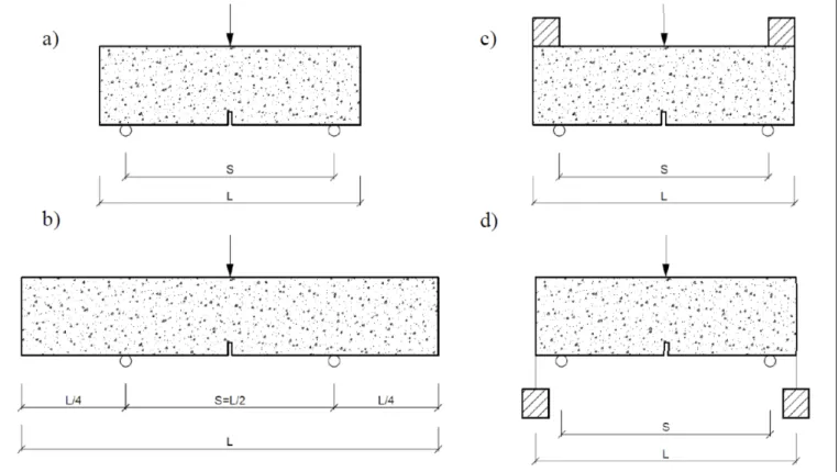
Hillerborg, 1985; JCI-S-001-2003, 2003; RILEM Technical Committee 50 FMC, 1985). There are different versions of the experimental setup of 3PBTs. If the supports are located close to the edges of the specimen, then after the opening of a certain critical crack (Fig. 1a), the specimen cracks due to gravity, independently of all other loads. In this case the total fracture energy cannot be measured, but it can be corrected during the evaluation of the results (JCI-S-001-2003, 2003;

RILEM Technical Committee 50 FMC, 1985). In order to balance the effect of self-weight, the measurement setup can also be designed so that the specimen extends significantly beyond the supports (Fig. 1b) or additional weights are placed at the ends of the beam (Fig. 1c and 1d) (Kaplan, 1961).

The adequate size of the specimen highly depends on the maximum aggregate size (d_max). Typically, even the smallest dimension of the specimen should be larger than 4 times d_max (JCI-S-001-2003, 2003); otherwise, the aggregate size will affect the value of the fracture energy.

The primary application of the notched 3PBT is to determine the fracture energy of concrete. However, the measurement setup is also suitable for determining additional mechanical parameters: flexural tensile strength, modulus of elasticity, and indirectly also the compressive strength. The aim of this paper is to present the calculation methods of the mechanical properties that can be determined from the test results of 3PBTs.

https://doi.org/10.32970/CS.2021.1.2

(2)

6 2021 •

CONCRETE STRUCTURES

2. EXPERIMENTAL DETAILS

2.1 Materials

During our tests, 7 types of aggregates were used. In normal concretes (NCs), the most typical river quartz gravel, sand and mined dolomite, limestone and andesite were used, while in lightweight concretes (LWCs), two types of expanded clay aggregates (ECAs) were applied.

The shape of quartz aggregate and ECA was rounded:

in case of quartz due to river fragmentation, while in case of ECA due to the technological process. The shape of the dolomite, limestone and andesite aggregate was angular due to the crushing process.

In case of the limestone aggregate, the body density was 2710 kg/m³, which was available from the data given by the mine. For the other aggregates, the body density was determined by own measurements. The body density of the quartz gravel aggregate was 2645 kg/m³, that of the dolomite aggregate was 2850 kg/m³, and that of the andesite aggregate was 2700 kg/m³. The body density of ECAs was 1465 kg/

m³ in case of type D1 and 1048 kg/m³in case of type D2.

In case of lightweight aggregates, their high porosity causes high water absorption, which also affects the water-cement ratio of the concrete mixture (Nemes and Józsa, 2006);

therefore, the ECAs were saturated with water. After 30 minutes of water absorption, the body density of type D1 was 1549 kg/m³, while that of type D2 was 1262 kg/m³. The amount of absorbed water was taken into account during the correction of the concrete mixtures.

The type of cement applied in our mixtures was CEM III/32.5 R containing slag. The water-cement ratio was 0.45. The consistency of fresh concretes was F4 (EN 12350- 5:2019, 2019) which was regulated by the addition of superplasticiser (BASF Glenium C300). The fraction 0/4 mm was quartz sand in all the mixtures when fraction 4/8 mm was

used. In order to make the comparison of the mixtures with different aggregates possible, it was important to evolve a similar aggregate skeleton; therefore, similar cement content, aggregate content and size distribution (0/4 mm 43%; 4/8 mm 57%) were applied. The concrete composition of different mixtures is summarised in Table 1.

The casted specimens were stored under water for 7 days and then in a climate chamber (temperature: 20 °C, relative humidity: 50 %). Tests of specimens were performed at 60 days of age.

2.2 Test equipment

In order to determine the fracture energy, crack mouth opening displacement (CMOD) controlled 3PBTs were carried out. The test setup is shown in Fig. 2. The applied CMOD controlled method is different from the previously recommended crosshead displacement controlled method (Hillerborg, 1985; RILEM Technical Committee 50 FMC, 1985), but it is accepted by many standards (EN 14651:2005+A1, 2007; JCI-S-001-2003, 2003). The force- CMOD curves derived by the two methods are the same (Lee and Lopez, 2014). The size of the applied specimens was 70x70x250 mm. Based on literature this size is big enough to make the effect of aggregate size negligeable in case of 8 mm maximum aggregate size (Fehérvári, Gálos, and Nehme, 2010b; Hillerborg, 1985; JCI-S-001-2003, 2003;

RILEM Technical Committee 50 FMC, 1985). The distance between the supports was 200 mm. The width of the notch was 4 mm, and its height was one sixth (12.5 mm) of the total height of the specimen. Crosshead displacement, CMOD and force were detected during the tests. During loading, the rate of CMOD was kept constant (0.01 mm/s).

The compressive strength of the concrete mixtures was determined by two methods. The compressive strength of cubes with the size of 150x150x150 mm was measured

Fig. 1: Notched 3PBTs: a) general; take into account the gravity b) with overhang, c) and d) with weights

(3)

CONCRETE STRUCTURES

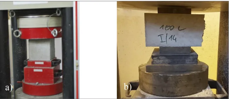
^•²⁰²¹ ⁷

according to the standard EN 12390-3 (EN 12390-3:2019, 2019). Compressive strength was also measured on half prisms previously subjected to 3PBT (Fig. 3) (Alimrani and Balazs, 2020; Lublóy, Balázs, and Czoboly, 2013), where the load was transferred by steel plates with the size of 70x70 mm, which was the same as the width of the prism.

Mechanical tests were extended by measurements of moisture content and apparent porosity, which were measured

on one half of the prisms. To determine moisture content, half prisms were dried in a drying furnace at 60 °C until constant mass. Initial moisture content could be calculated by the difference between the original and the dried mass.

After drying, the specimens were stored under water until constant mass, therefore the amount of water uptake could be measured, and the volume of open pores could be determined (EN 1936:2007, 2007).

Table 1: Concrete mix designs for 1 m³ (quantities are in kg)

Unit weight Mixture symbol

4S 4S8Q 4D 4S8D 4S8L 4S8A 4S8D1 4S8D2

Aggregate sand (0/4 mm) 1391 782 - 782 782 782 782 782

quartz (4/8 mm) - 1037 - - - -

dolomite (0/4 mm) - - 1499 - - - - -

dolomite (4/8 mm) - - - 1118 - - - -

limestone (4/8 mm) - - - - 1063 - - -

andesite (4/8 mm) - - - 1059 - -

expanded clay D1 (4/8 mm) - - - 574* -

expanded clay D2 (4/8 mm) - - - 411*

Cement (CEM III/32.5 R): 600 390 600 390 390 390 390 390

Water: 270 175 270 175 175 175 175 175

w/c ratio 0.45 0.45 0.45 0.45 0.45 0.45 0.45 0.45

Superplasticizer: 0.3 0.78 0.45 1.79 2.4 3.5 0.4 0.2

* calculated with dry body density of aggregate

Fig. 2: Setup of the 3PBT

Fig. 3: Compressive strength test: a) cube; b) half prism

(4)

8 2021 •

CONCRETE STRUCTURES

3. RESULTS AND DISCUSSION

3.1 Body density, moisture content and apparent porosity

Dry body density values (Table 2) of the mixtures with ECA (4S8D1, 4S8D2) were lower than 2000 kg/m³, therefore they could be considered as LWC (fib BULLETIN 8, 2000;

fib MC2010, 2013). As expected, the apparent porosity of LWC mixtures was high due to the high porosity of aggregate particles. The apparent porosity of the mixture containing quartz sand only (4S) and dolomite sand only (4D) was also high. The mixtures with dolomite gravel (4S8D) and andesite gravel (4S8A) had the highest body density and consequently the lowest apparent porosity and moisture content.

3.2 Compressive strength

The fib Model Code 2010 (fib MC2010, 2013) calculates the mechanical parameters by using the compressive strength of concrete. Therefore, in addition to 3PBTs, compressive strength tests were also performed using cubes and half prisms previously subjected to 3PBT. The results of the measurements are summarised in Table 2 and Fig. 4.

As expected, the LWCs had the lowest compressive strength. The compressive strength of the mixture with lower body density ECA (4SD2) was significantly lower than that of the mixture with higher body density ECA (4SD1). The mixtures with andesite gravel (4S8A) and with limestone gravel (4S8L) had the highest compressive strength, which is well reflected in the high body density of both mixtures.

The results show that the values measured on cubes and on half prisms were close to each other. Typically, the variance

of the values measured on half prisms was larger than that of the values measured on cubes. Based on the value pairs shown, the compressive strength values measured on half prisms were lower than the values measured on cubes if the latter was below 66 N/mm². Above 66 N/mm² the prisms had higher compressive strength.

3.3 Flexural tensile strength

From the data measured during the notched 3PBTs the flexural tensile strength of the mixture could also be directly calculated by using the following formula:

𝑓𝑓𝑓𝑓

𝑐𝑐𝑐𝑐𝑐𝑐𝑐𝑐,𝑓𝑓𝑓𝑓𝑓𝑓𝑓𝑓

=

_{2𝑏𝑏𝑏𝑏ℎ}^{3𝐹𝐹𝐹𝐹𝐹𝐹𝐹𝐹}₂(EN 14651:2005+A1,2007)

(1)

𝑓𝑓𝑓𝑓

𝑐𝑐𝑐𝑐𝑐𝑐𝑐𝑐𝑐𝑐𝑐𝑐,𝑓𝑓𝑓𝑓𝑓𝑓𝑓𝑓

=

2.12∗ln (1+0.1(𝑓𝑓𝑓𝑓_{𝑐𝑐𝑐𝑐𝑐𝑐𝑐𝑐}+∆𝑓𝑓𝑓𝑓))

𝛼𝛼𝛼𝛼𝑓𝑓𝑓𝑓𝑓𝑓𝑓𝑓 (fib MC2010,2013)

(2)

𝛼𝛼𝛼𝛼

𝑓𝑓𝑓𝑓𝑓𝑓𝑓𝑓

=

_{1+0.06𝑏𝑏𝑏𝑏}^{0.06𝑏𝑏𝑏𝑏}^0,7_0,7(fib MC2010,2013)

(3)

𝑓𝑓𝑓𝑓

𝑓𝑓𝑓𝑓𝑐𝑐𝑐𝑐𝑐𝑐𝑐𝑐𝑐𝑐𝑐𝑐,𝑓𝑓𝑓𝑓𝑓𝑓𝑓𝑓

=

^{𝜇𝜇𝜇𝜇}^{𝑓𝑓𝑓𝑓}^{∗0.3(𝑓𝑓𝑓𝑓}_{𝛼𝛼𝛼𝛼} ^{𝑐𝑐𝑐𝑐𝑐𝑐𝑐𝑐}⁾^2/3

𝑓𝑓𝑓𝑓𝑓𝑓𝑓𝑓 (fib MC2010,2013)

(4)

𝜇𝜇𝜇𝜇

𝑓𝑓𝑓𝑓

= (0.4 + 0.6

₂₂₀₀^{𝜌𝜌𝜌𝜌}

)

(fib MC2010,2013)

(5) 𝐸𝐸𝐸𝐸 =

6𝐹𝐹𝐹𝐹𝑆𝑆𝑆𝑆𝑉𝑉𝑉𝑉₁(𝑆𝑆𝑆𝑆 𝐻𝐻𝐻𝐻⁄ )

𝐶𝐶𝐶𝐶_{𝑖𝑖𝑖𝑖}𝐻𝐻𝐻𝐻²𝑏𝑏𝑏𝑏 (Surendra,1990)

(6)

𝑉𝑉𝑉𝑉

₁

�

^{𝑆𝑆𝑆𝑆}_{𝐻𝐻𝐻𝐻}

� = 0.76 − 2.28 �

_{𝐻𝐻𝐻𝐻}^{𝑆𝑆𝑆𝑆}

� + 3.87 �

�

²

− 2.04 �

�

³

+

_(1−�^0.66𝑎𝑎𝑎𝑎 𝐻𝐻𝐻𝐻�)²

(Tada, Paris, and Irwin,2000)

(7)

𝐸𝐸𝐸𝐸

_{𝑐𝑐𝑐𝑐}

= 𝐸𝐸𝐸𝐸

_{𝑐𝑐𝑐𝑐0}

𝛼𝛼𝛼𝛼

_{𝐸𝐸𝐸𝐸}

(

^{𝑓𝑓𝑓𝑓}₁₀^{𝑐𝑐𝑐𝑐𝑐𝑐𝑐𝑐}

)

^1/3(fib MC2010,2013)

(8)

𝐸𝐸𝐸𝐸

𝑓𝑓𝑓𝑓𝑐𝑐𝑐𝑐

= 𝜇𝜇𝜇𝜇

𝐸𝐸𝐸𝐸

𝑐𝑐𝑐𝑐 (fib MC2010,2013)

(9)

𝜇𝜇𝜇𝜇

_{𝐸𝐸𝐸𝐸}

= (

₂₂₀₀^{𝜌𝜌𝜌𝜌}

)

² (fib MC2010,2013)

(10) 𝐺𝐺𝐺𝐺

_{𝐹𝐹𝐹𝐹}

=

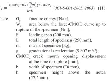
^{0.75𝑊𝑊𝑊𝑊}⁰^+0.75�^{𝑆𝑆𝑆𝑆}^{𝐿𝐿𝐿𝐿}𝑐𝑐𝑐𝑐�𝑔𝑔𝑔𝑔∗𝐶𝐶𝐶𝐶𝐶𝐶𝐶𝐶𝐶𝐶𝐶𝐶𝐶𝐶𝐶𝐶𝑐𝑐𝑐𝑐

𝑏𝑏𝑏𝑏∗ℎ (JCI-S-001-2003,2003)

(11)

𝐺𝐺𝐺𝐺

𝐹𝐹𝐹𝐹

= 73𝑓𝑓𝑓𝑓

𝑐𝑐𝑐𝑐𝑐𝑐𝑐𝑐0.18(fib MC2010,2013)

(12)

𝐺𝐺𝐺𝐺

_{𝐹𝐹𝐹𝐹,𝑓𝑓𝑓𝑓}

= 𝐺𝐺𝐺𝐺

_{𝑓𝑓𝑓𝑓0𝐴𝐴𝐴𝐴}

+ 16𝑓𝑓𝑓𝑓

𝑓𝑓𝑓𝑓𝑐𝑐𝑐𝑐𝑐𝑐𝑐𝑐𝑐𝑐𝑐𝑐(fib MC2010,2013)

(13)

𝐺𝐺𝐺𝐺

𝐹𝐹𝐹𝐹

= 𝐺𝐺𝐺𝐺

𝐹𝐹𝐹𝐹0

(𝑓𝑓𝑓𝑓

𝑐𝑐𝑐𝑐𝑐𝑐𝑐𝑐

/𝑓𝑓𝑓𝑓

𝑐𝑐𝑐𝑐𝑐𝑐𝑐𝑐0

)

^0.7^(CEB-FIP,¹⁹⁹³⁾

(14)

𝐺𝐺𝐺𝐺

𝐹𝐹𝐹𝐹,𝑁𝑁𝑁𝑁𝐶𝐶𝐶𝐶,8

= 71.7𝑓𝑓𝑓𝑓

𝑐𝑐𝑐𝑐𝑐𝑐𝑐𝑐,0.5𝑝𝑝𝑝𝑝𝑝𝑝𝑝𝑝𝑝𝑝𝑝𝑝𝑝𝑝𝑝𝑝𝑐𝑐𝑐𝑐0.18

(15)

𝐺𝐺𝐺𝐺

= 53.4𝑓𝑓𝑓𝑓

(16)

𝐺𝐺𝐺𝐺

𝐹𝐹𝐹𝐹,𝐿𝐿𝐿𝐿𝑊𝑊𝑊𝑊𝐶𝐶𝐶𝐶

= 40.1𝑓𝑓𝑓𝑓

(17)

(1) where: f_ct,fl flexural tensile strength [N/mm²],

F the force of rupture [N]

S loading span (200 mm), b width of specimen (70 mm), h specimen’s height above the notch

(57.5 mm).

The flexural tensile strength values calculated from the data measured during the notched 3PBTs are summarised in Table 2.

The fib Model Code 2010 provides a formula for the calculation of the pure tensile strength of concrete, which can be converted to flexural tensile strength by a factor depending on the width of the specimen (α_fl). The formula is as follows, if the concrete strength class is higher than C50/60:

𝑓𝑓𝑓𝑓𝑐𝑐𝑐𝑐𝑐𝑐𝑐𝑐,𝑓𝑓𝑓𝑓𝑓𝑓𝑓𝑓 =_{2𝑏𝑏𝑏𝑏ℎ}^{3𝐹𝐹𝐹𝐹𝐹𝐹𝐹𝐹}₂(EN 14651:2005+A1,2007) (1)

𝑓𝑓𝑓𝑓𝑐𝑐𝑐𝑐𝑐𝑐𝑐𝑐𝑐𝑐𝑐𝑐,𝑓𝑓𝑓𝑓𝑓𝑓𝑓𝑓 =2.12∗ln (1+0.1(𝑓𝑓𝑓𝑓_{𝑐𝑐𝑐𝑐𝑐𝑐𝑐𝑐}+∆𝑓𝑓𝑓𝑓))

𝛼𝛼𝛼𝛼𝑓𝑓𝑓𝑓𝑓𝑓𝑓𝑓 (fib MC2010,2013) (2)

𝛼𝛼𝛼𝛼𝑓𝑓𝑓𝑓𝑓𝑓𝑓𝑓 =_{1+0.06𝑏𝑏𝑏𝑏}^{0.06𝑏𝑏𝑏𝑏}^0,7_0,7(fib MC2010,2013) (3)

𝑓𝑓𝑓𝑓𝑓𝑓𝑓𝑓𝑐𝑐𝑐𝑐𝑐𝑐𝑐𝑐𝑐𝑐𝑐𝑐,𝑓𝑓𝑓𝑓𝑓𝑓𝑓𝑓 = ^{𝜇𝜇𝜇𝜇}^{𝑓𝑓𝑓𝑓}^{∗0.3(𝑓𝑓𝑓𝑓}_{𝛼𝛼𝛼𝛼}_{𝑓𝑓𝑓𝑓𝑓𝑓𝑓𝑓}^{𝑐𝑐𝑐𝑐𝑐𝑐𝑐𝑐}⁾^2/3(fib MC2010,2013) (4)

𝜇𝜇𝜇𝜇𝑓𝑓𝑓𝑓 = (0.4 + 0.6₂₂₀₀^{𝜌𝜌𝜌𝜌} ) (fib MC2010,2013) (5) 𝐸𝐸𝐸𝐸 = 6𝐹𝐹𝐹𝐹𝑆𝑆𝑆𝑆𝑉𝑉𝑉𝑉1(𝑆𝑆𝑆𝑆 𝐻𝐻𝐻𝐻⁄ )

𝐶𝐶𝐶𝐶_{𝑖𝑖𝑖𝑖}𝐻𝐻𝐻𝐻²𝑏𝑏𝑏𝑏 (Surendra,1990) (6)

𝑉𝑉𝑉𝑉1�^{𝑆𝑆𝑆𝑆}_{𝐻𝐻𝐻𝐻}�= 0.76−2.28�_{𝐻𝐻𝐻𝐻}^{𝑆𝑆𝑆𝑆}�+ 3.87�_{𝐻𝐻𝐻𝐻}^{𝑆𝑆𝑆𝑆}�²−2.04�_{𝐻𝐻𝐻𝐻}^{𝑆𝑆𝑆𝑆}�³+_(1−�^0.66𝑎𝑎𝑎𝑎 𝐻𝐻𝐻𝐻�)²

(Tada, Paris, and Irwin,2000) (7)

𝐸𝐸𝐸𝐸𝑐𝑐𝑐𝑐= 𝐸𝐸𝐸𝐸𝑐𝑐𝑐𝑐0𝛼𝛼𝛼𝛼𝐸𝐸𝐸𝐸(^{𝑓𝑓𝑓𝑓}₁₀^{𝑐𝑐𝑐𝑐𝑐𝑐𝑐𝑐})^1/3(fib MC2010,2013) (8)

𝐸𝐸𝐸𝐸𝑓𝑓𝑓𝑓𝑐𝑐𝑐𝑐 = 𝜇𝜇𝜇𝜇𝐸𝐸𝐸𝐸𝐸𝐸𝐸𝐸𝑐𝑐𝑐𝑐(fib MC2010,2013) (9)

𝜇𝜇𝜇𝜇𝐸𝐸𝐸𝐸 = (₂₂₀₀^{𝜌𝜌𝜌𝜌} )²(fib MC2010,2013) (10) 𝐺𝐺𝐺𝐺𝐹𝐹𝐹𝐹 =^{0.75𝑊𝑊𝑊𝑊}⁰^+0.75�^{𝑆𝑆𝑆𝑆}^{𝐿𝐿𝐿𝐿}𝑐𝑐𝑐𝑐�𝑔𝑔𝑔𝑔∗𝐶𝐶𝐶𝐶𝐶𝐶𝐶𝐶𝐶𝐶𝐶𝐶𝐶𝐶𝐶𝐶𝑐𝑐𝑐𝑐

𝑏𝑏𝑏𝑏∗ℎ (JCI-S-001-2003,2003) (11)

𝐺𝐺𝐺𝐺𝐹𝐹𝐹𝐹 = 73𝑓𝑓𝑓𝑓𝑐𝑐𝑐𝑐𝑐𝑐𝑐𝑐0.18(fib MC2010,2013) (12)

𝐺𝐺𝐺𝐺𝐹𝐹𝐹𝐹,𝑓𝑓𝑓𝑓 =𝐺𝐺𝐺𝐺𝑓𝑓𝑓𝑓0𝐴𝐴𝐴𝐴+ 16𝑓𝑓𝑓𝑓𝑓𝑓𝑓𝑓𝑐𝑐𝑐𝑐𝑐𝑐𝑐𝑐𝑐𝑐𝑐𝑐(fib MC2010,2013) (13)

𝐺𝐺𝐺𝐺𝐹𝐹𝐹𝐹 =𝐺𝐺𝐺𝐺𝐹𝐹𝐹𝐹0(𝑓𝑓𝑓𝑓𝑐𝑐𝑐𝑐𝑐𝑐𝑐𝑐/𝑓𝑓𝑓𝑓𝑐𝑐𝑐𝑐𝑐𝑐𝑐𝑐0)^0.7^(CEB-FIP,¹⁹⁹³⁾ (14)

𝐺𝐺𝐺𝐺𝐹𝐹𝐹𝐹,𝑁𝑁𝑁𝑁𝐶𝐶𝐶𝐶,8 = 71.7𝑓𝑓𝑓𝑓𝑐𝑐𝑐𝑐𝑐𝑐𝑐𝑐,0.5𝑝𝑝𝑝𝑝𝑝𝑝𝑝𝑝𝑝𝑝𝑝𝑝𝑝𝑝𝑝𝑝𝑐𝑐𝑐𝑐0.18 (15)

𝐺𝐺𝐺𝐺𝐹𝐹𝐹𝐹,𝑁𝑁𝑁𝑁𝐶𝐶𝐶𝐶,4 = 53.4𝑓𝑓𝑓𝑓𝑐𝑐𝑐𝑐𝑐𝑐𝑐𝑐,0.5𝑝𝑝𝑝𝑝𝑝𝑝𝑝𝑝𝑝𝑝𝑝𝑝𝑝𝑝𝑝𝑝𝑐𝑐𝑐𝑐0.18 (16)

𝐺𝐺𝐺𝐺𝐹𝐹𝐹𝐹,𝐿𝐿𝐿𝐿𝑊𝑊𝑊𝑊𝐶𝐶𝐶𝐶 = 40.1𝑓𝑓𝑓𝑓𝑐𝑐𝑐𝑐𝑐𝑐𝑐𝑐,0.5𝑝𝑝𝑝𝑝𝑝𝑝𝑝𝑝𝑝𝑝𝑝𝑝𝑝𝑝𝑝𝑝𝑐𝑐𝑐𝑐0.18 (17)

(2)

𝑓𝑓𝑓𝑓

𝑐𝑐𝑐𝑐𝑐𝑐𝑐𝑐,𝑓𝑓𝑓𝑓𝑓𝑓𝑓𝑓

=

_{2𝑏𝑏𝑏𝑏ℎ}^{3𝐹𝐹𝐹𝐹𝐹𝐹𝐹𝐹}₂(EN 14651:2005+A1,2007)

(1)

𝑓𝑓𝑓𝑓

𝑐𝑐𝑐𝑐𝑐𝑐𝑐𝑐𝑐𝑐𝑐𝑐,𝑓𝑓𝑓𝑓𝑓𝑓𝑓𝑓

=

2.12∗ln (1+0.1(𝑓𝑓𝑓𝑓_{𝑐𝑐𝑐𝑐𝑐𝑐𝑐𝑐}+∆𝑓𝑓𝑓𝑓))

𝛼𝛼𝛼𝛼_{𝑓𝑓𝑓𝑓𝑓𝑓𝑓𝑓} (fib MC2010,2013)

(2)

𝛼𝛼𝛼𝛼

_{𝑓𝑓𝑓𝑓𝑓𝑓𝑓𝑓}

=

_{1+0.06𝑏𝑏𝑏𝑏}^{0.06𝑏𝑏𝑏𝑏}^0,7_0,7(fib MC2010,2013)

(3)

𝑓𝑓𝑓𝑓

𝑓𝑓𝑓𝑓𝑐𝑐𝑐𝑐𝑐𝑐𝑐𝑐𝑐𝑐𝑐𝑐,𝑓𝑓𝑓𝑓𝑓𝑓𝑓𝑓

=

^{𝜇𝜇𝜇𝜇}^{𝑓𝑓𝑓𝑓}^{∗0.3(𝑓𝑓𝑓𝑓}_{𝛼𝛼𝛼𝛼} ^{𝑐𝑐𝑐𝑐𝑐𝑐𝑐𝑐}⁾^2/3

𝑓𝑓𝑓𝑓𝑓𝑓𝑓𝑓 (fib MC2010,2013)

(4)

𝜇𝜇𝜇𝜇

_{𝑓𝑓𝑓𝑓}

= (0.4 + 0.6

₂₂₀₀^{𝜌𝜌𝜌𝜌}

)

(fib MC2010,2013)

(5) 𝐸𝐸𝐸𝐸 =

6𝐹𝐹𝐹𝐹𝑆𝑆𝑆𝑆𝑉𝑉𝑉𝑉₁(𝑆𝑆𝑆𝑆 𝐻𝐻𝐻𝐻⁄ )

𝐶𝐶𝐶𝐶_{𝑖𝑖𝑖𝑖}𝐻𝐻𝐻𝐻²𝑏𝑏𝑏𝑏 (Surendra,1990)

(6)

𝑉𝑉𝑉𝑉

₁

�

� = 0.76 − 2.28 �

� + 3.87 �

�

²

− 2.04 �

�

³

+

_(1−�^0.66𝑎𝑎𝑎𝑎 𝐻𝐻𝐻𝐻�)²

(Tada, Paris, and Irwin,2000)

(7)

𝐸𝐸𝐸𝐸

𝑐𝑐𝑐𝑐

= 𝐸𝐸𝐸𝐸

𝑐𝑐𝑐𝑐0

𝛼𝛼𝛼𝛼

𝐸𝐸𝐸𝐸

(

^{𝑓𝑓𝑓𝑓}₁₀^{𝑐𝑐𝑐𝑐𝑐𝑐𝑐𝑐}

)

^1/3(fib MC2010,2013)

(8)

𝐸𝐸𝐸𝐸

𝑓𝑓𝑓𝑓𝑐𝑐𝑐𝑐

= 𝜇𝜇𝜇𝜇

𝐸𝐸𝐸𝐸

𝑐𝑐𝑐𝑐 (fib MC2010,2013)

(9)

𝜇𝜇𝜇𝜇

_{𝐸𝐸𝐸𝐸}

= (

₂₂₀₀^{𝜌𝜌𝜌𝜌}

)

² (fib MC2010,2013)

(10) 𝐺𝐺𝐺𝐺

𝐹𝐹𝐹𝐹

=

^{0.75𝑊𝑊𝑊𝑊}⁰^+0.75�^{𝑆𝑆𝑆𝑆}^{𝐿𝐿𝐿𝐿}𝑐𝑐𝑐𝑐�𝑔𝑔𝑔𝑔∗𝐶𝐶𝐶𝐶𝐶𝐶𝐶𝐶𝐶𝐶𝐶𝐶𝐶𝐶𝐶𝐶_{𝑐𝑐𝑐𝑐}

𝑏𝑏𝑏𝑏∗ℎ (JCI-S-001-2003,2003)

(11)

𝐺𝐺𝐺𝐺

_{𝐹𝐹𝐹𝐹}

= 73𝑓𝑓𝑓𝑓

_{𝑐𝑐𝑐𝑐𝑐𝑐𝑐𝑐}^0.18(fib MC2010,2013)

(12)

𝐺𝐺𝐺𝐺

_{𝐹𝐹𝐹𝐹,𝑓𝑓𝑓𝑓}

= 𝐺𝐺𝐺𝐺

_{𝑓𝑓𝑓𝑓0𝐴𝐴𝐴𝐴}

+ 16𝑓𝑓𝑓𝑓

𝑓𝑓𝑓𝑓𝑐𝑐𝑐𝑐𝑐𝑐𝑐𝑐𝑐𝑐𝑐𝑐(fib MC2010,2013)

(13)

𝐺𝐺𝐺𝐺

_{𝐹𝐹𝐹𝐹}

= 𝐺𝐺𝐺𝐺

_{𝐹𝐹𝐹𝐹0}

(𝑓𝑓𝑓𝑓

_{𝑐𝑐𝑐𝑐𝑐𝑐𝑐𝑐}

/𝑓𝑓𝑓𝑓

_{𝑐𝑐𝑐𝑐𝑐𝑐𝑐𝑐0}

)

^0.7^(CEB-FIP,¹⁹⁹³⁾

(14)

𝐺𝐺𝐺𝐺

= 71.7𝑓𝑓𝑓𝑓

(15)

𝐺𝐺𝐺𝐺

= 53.4𝑓𝑓𝑓𝑓

(16)

𝐺𝐺𝐺𝐺

𝐹𝐹𝐹𝐹,𝐿𝐿𝐿𝐿𝑊𝑊𝑊𝑊𝐶𝐶𝐶𝐶

= 40.1𝑓𝑓𝑓𝑓

(17)

(3) where: f_ctm,fl mean flexural tensile strength [N/mm²], f_ck characteristic compressive

strength [N/mm²], Δf 8 N/mm²,

b width of specimen (70 mm).

It can be seen in the formula (Eq. 2) that 8 N/mm² is added to the characteristic value of the compressive strength of the concrete, which will thus correspond to the mean compressive strength.

In the case of LWC, the recommended relation also takes into account the body density of the concrete:

Table 2. Average values of measured non-mechanical and mechanical properties of the mixtures (each value is the average of 3 or 4 measurements)

Mixture Dry body density [kg/m³]

Moisture content

[%]

Apparent porosity

[%]

Compressive strength

[N/mm²] Flexural tensile strength [N/mm²]

Modulus of elas-

ticity [N/mm²] Fracture energy [N/m]

cube half prism