VS-type Stabilization of MRAC Controllers Using Robust Fixed Point Transformations
Ter´ez A. V´arkonyi∗, J´ozsef K. Tar†, Imre J. Rudas†, Istv´an Kr´omer‡
∗Doctoral School of Applied Informatics, John von Neumann Faculty of Informatics Obuda University´
96/B B´ecsi ´ut, Budapest, H-1034, Hungary varkonyi.teri@phd.uni-obuda.hu
†Institute of Intelligent Engineering Systems, John von Neumann Faculty of Informatics Obuda University´
96/B B´ecsi ´ut, Budapest, H-1034, Hungary tar.jozsef@nik.uni-obuda.hu, rudas@nik.uni-obuda.hu
‡Kand´o K´alm´an Faculty of Electrical Engineering Obuda University´
15 Tavaszmez˝o ´ut, Budapest, H-1084, Hungary kromer.istvan@kvk.uni-obuda.hu
Abstract—Nowadays, control of dynamical systems with uncer- tainties is a common problem. Many sulutions can be found in the literature, one of these methods is the family of Robust Fixed Point Transformations (RFPT) with local basin of attraction.
The method is based on the idea that if someone has to use an approximate model in a control task, there is a function which, locally converging to the right solution, can reduce the disadvantages of the approximation. In this paper, authors show that though RFPT can loose its local convergensity, it can still improve a simple controller’s results and this improvement makes the controller’s behavior very similar to that of a sliding mode controller. The similarity includes the so called chattering effect, but a simple smoothing algorithm is also introuced to minimize the fluctuation of the control signal.
I. INTRODUCTION
In the 19th century stability of dynamical systems was a problematic subject for the scientists. It was sometimes very elaborate to determine whether a system was stable or not and only a few results were at hand to answer these questions. One of the first breakthroughs was made by Aleksandr Lyapunov in 1892. In his PhD dissertation [1] he introduced an approach, called Lyapunov’s “direct” method, in which on the basis of relatively simple estimations, stability (either global or local, common, exponential, or asymptotic) could be determined without obtaining and studying the solutions of the equations of motion. (It is well known that the most of the practically occurring problems do not have analytical solutions in closed form, while the numerical solutions are normally valid only for the limited time-span of investigations and without deeper mathematical background their results cannot be extrapolated.) Lyapunov’s work was translated to English approximately 75 years later, in the 20thcentury [2] and since that it has become
the possibly most significant mathematical tool for designing stable controllers for linear and nonlinear systems (for some examples [3]-[11]).
The advantage of the Sliding Mode Control (SMC) is its simplicity, characterized by robustness which makes the con- troller able to handle dynamical systems with heavy uncertain conditions. In sliding mode, SMC does not just behave as a reduced order system with respect to the original system, but is insensitive to uncertainities and disturbances. On the contrary it has a main disadvantage, the so-called chattering effect, which demands the system to fluctuate so quick that it might get damaged in short time because of the stress [12].
Robust Fixed Point Transformation is a method based on an idea that if someone has to use an approximate model in a control task, there is a function which, locally converging to the right solution, can reduce the disadvantages of the approximation. As included in its name, RFPT is characterized by robustness and it has the ability to handle rough approxima- tions also, without increasing the performance of the controller considerably. These properties make RFPT very similar to SMC.
Previous researches showed that in fact there are many opportunities to choose this function, the only constraint is that is has to be contractive [13]. The other advantage, researches showed, that the improvement achieved by this function can be increased by applying small modifcations to this function during the controlling process [14].
In this paper, a new behavior of RFPT is introduced. As mentioned above, the method is based on a locally convergent function. As the simulations show, if this function looses its local convergensity, instead of loosing stability, it makes
the controller behave like a Sliding Mode Controller which can still reduce the disadvantages of the appproximation. The similarity includes the chattering effect, but an additional smoothing algotihm is introduced which reduces the fluctu- ation to minimal or in some cases it dissolves it, so the controller is not exposed to high stress level.
In the paper, the simulation task is controlling a higly nonlinear Φ6 Van der Pol oscillator. For comparison, sim- ulations are made by a simple (nonadaptive) PID and an (adaptive) RFPT-based PID controller. As the simultions show with loosing convergencity the RPPT can still reduce the nonadaptive controller’s results with more than one order without noticeable chattering.
The paper is organized as follows. Section II is devoted to the expected-observed response sceme and the fixed point transformation with parameter tuning and the smoothing algo- rithm. In Section III the Van der Pol oscillator is explained in details. Section IV shows the simulation results and finally, in Section V the conclusions are summarized.
II. THE EXPECTED-OBSERVED RESPONSE SCEME AND THE FIXED POINT TRANSFORMATION
Most of the control tasks can be formulated by an equation expressing a correspondenceϕbetween the appropriate “exci- tation”Qof the system and a prescribed responserd. With the help of the inverse dynamic modelQ=ϕ(rd), this excitation can be computed. But here comes the first difficulty because this model is not exact or complete so it generates a realized response rr which is determined by the system’s dynamics ψ and differs from rd: rr ≡ ψ(ϕ(rd)) ≡f(rd)6= rd. Gen- erally ϕ()and ψ() contain hidden parameters corresponding to the dynamic model of the system and unknown external dynamic forces refer to them. That’s why we can’t define their composition f() exactly. The second difficulty is that:
unfortunately, due to phenomenological reasons the controller can manipulate the input value (got from the previous step’s output with feedback)rd =f(r∗) so a method is needed to find the deformed inputx∗.
The iterative fixed point transformation [13] is very useful because if we can find a proper Ψ(r) function which fixed point is the wanted r∗: Ψ(r∗) = r∗, then the problem can be easily solved. Thanks to Banach fixed point theorem [15]
this question can effortlessly be resolved via simple iteration as long as the iteration is convergent. The following iterative fixed point searching algorithm proves that if a sequence constructed by theΨfunction is convergent than the limit value is the fixed point of the mapping. In the next few paragraphs the authors show a proof of this statement.
Take the next iterative sequence: x0, x1 = Ψ(x0), ... , xn+1 = Ψ(xn). Take the set of the real numbers R as a linear normed space where the two operations are the common addition and the multiplication with real numbers and the norm is the absolute value. In this case, this space is complete, and it is Banach space, too.
In Banach spaces the Cauchy Sequences are convergent so in the next step a satisfactory condition is needed of (xn)
being a Cauchy Sequence. This condition is the contractivity ofΨ()which means∃ 0≤M <1 ∀a, b∈R|Ψ(a)−Ψ(b)| ≤ M|a−b|. In this case ∀L∈N
|xn+L−xn|=|Ψ(xn+L−1)−Ψ(xn−1)| ≤
...≤Mn|xL−x0| →0as n→ ∞ (1) This inequality guarantees that (xn) is a Cauchy Sequence.
The next step in the proof is securing the contractivity of the Ψ() function. To be able to do that we have to limit the absolute value of its derivative|Ψ0| ≤M <1 because in this case
|Ψ(a)−Ψ(b)|=|Rb
a Ψ0(x)dx| ≤ Rb
a|Ψ0(x)|dx≤M|a−b| (2) The last step is prooving that if the previous sequence is convergent, than Ψ()has has a fixed point which is the limit value of the{xn}series. Assume that{xn}converges to some x∗. Then if we suppose thatΨis continuous then
|Ψ(x∗)−x∗| ≤ |Ψ(x∗)−xn|+|xn−x∗|=
|Ψ(x∗)−Ψ(xn−1)|+|xn−x∗| (3) It is obvious from Eq. (3) that Ψ(x∗) =x∗ because on the right hand side both terms converge to zero as n→ ∞.
This means that ifΨis flat enough around the fixed point the iteration will converge to it. The next task is the construction of the proper mapping Ψ. Based on previous researches an improved function is proposed:
G x, xd
= (x+K)×
× 1 +Btanh A
f(x)−xd
−K wheref(x∗) =xd and G0 x, xd
= (x+K)ABf0(x) cosh2(A[f(x)−xd])
+ +1 +Btanh A
f(x)−xd
(4)
The equation has three free parameters A, B, and K. With the proper manipulation the necessary limitation G0 x∗, xd
<1 can be guaranteed. It has two fixed points, the wanted x∗ and a false one −K, which can be easily excluded in the knowledge ofK.Gis robust with the respect to the fluctuation of the unknownf function. This robustness is a consequence of the strong nonlinear saturation of the sigmoid functiontanh(), and can be approximately investigated by the use of an affine approximation of f(x) in the vicinity ofx∗. The iteration of G converge with a considerable speed even nearby x∗ and because of its robustness the f function has less influence on the behavior of it.
So if we assume that xd varies slowly which means it is almost constant then Ψ(x) = G(x, xd) is a proper choice.
Qualitatively it can be stated that a small value of the param- eter A opens a wide “window” in the vicinity of the realized response, while parameter K can yield an additional shift to speed up the convergence. Practically these parameters can be set via simulations. By the use of a simple PD-type controller one can observe the order of magnitude of the desired and simulated responses, B = ±1 can be used and A and K
can be set accordingly. Normally very big|K|and very small positiveAcan be chosen. Furthermore, any bounded, strictly monotone increasing differentiable σ(x) function that also fulfills theσ(0) = 0property is appropriate for our purposes, e.g.σ(x) =x/(1 +|x|).
A. Parameter tuning for RFPT
However, the observation that a particular value for A rather influence the speed of convergence than the fact of convergencity itself, instead of a singleA, (4) can be calculated for a set of possible {Ai} values and the output can be determined as a weighted sum of the possible propositions belonging to the variousAis as
x(n+ 1) =Pm
i=1wixi(n+ 1) xi(n+ 1) = (xn+K)×
× 1 +Btanh Ai
f(xn)−xdn+1
−K
(5) in which thewi>0weighting factors can be determined as
˜
wi=ϑ(i, ζ, ς,∆) = 1/(ς2+ (i∆−ζ)2) wi=Pmw˜i
j=1w˜j
(6) that corresponds to a weighted sum of various propositions.
After setting and fixing the ς,∆ parameters and moving the center of the membership function in time with constant velocity ζ >˙ 0, a tuned membership function is obtained in which the weights of thei∆< ζ Ais decrease while that of the i∆> ζ Ais increase. The greatest weight is given to thoseAj
for which|j∆−ζ|is minimal. In generalζ >˙ 0corresponds to increasing, whileζ <˙ 0pertains to decreasing weights. On this basis the following simple tuning is applied: ζ = ±vζ with constantvζ >0 value. If a givenζ˙cause that the sum of the absolute response error decrease during five control steps, it is kept. Otherwise its sign is changed. It worths noting that the ζ → ±∞ should result in the equalization of the voting weights so this mechanism automatically keepsζ finite.
The adaptive control parameters in the simulation are as fol- lows:K= 7000,B=−1, and{Ai= 10−3+i∆|i= 0, ...,2},
∆ = 0.05,ς = 1, andζ= 1.
B. Reduction of chattering
As it is told in Section I, the controller is based on a locally convergent function 4 which sometimes can loose its convergensity, because it is unstable near to its fixed point. In this case when it gets an input very close to its fixed point, it pushes the output far. In this case the next input is not so close to the fixed point. The function keeps pushing its output away until it gets a far enough input, which is not in the unstable zone. If the input gets out of the unstable zone, it is converged again to the fixed point. This behaviour makes the controller similar to the Sliding Mode Controllers. The fluctuations observed in the control signal are in the order of magnitude ofK, which is one of the three free parameters of 4. This means a huge chattering.
To avoid the stress caused by the fluctuation of the control signal, a simple algorithm is proposed:
• Put the output of function G into a sigmoid with the property σ(0) = 0 by the use of a new parameter Kctrl Kvssm >0 as xi+1 =KvssmσG(x
i|rdi) Kvssm
(in the forthcoming simulationsKvssm= 700was used);
• Observe the change in the sign of the exerted forces by refreshing the content of a forgetting buffer as QBufi+1 = βQBufi +Qi−2Qi−1with someβ∈(0,1); If the content of this buffer becomes negative strong chattering occurs since the sign of the exerted force varies in each control step;
• IfQBuf >0apply the fine tuning with the voting weights as in Subsection II-A; If QBuf < 0 then stop the fine tuning and rigidly push the possibleAi parameters in the negative direction (with ∀iAi>0).
As a result the chattering is kept at bay while Ai values decrease to the necessary extent for restoring the convergence and completely ceasing any chattering. In the sequel at first the Φ6 Van der Pol oscillator is described then this solution will be used and investigated via simulations.
III. THE MODEL OF THEΦ6VAN DERPOL OSCILLATOR AND THEPIDCONTROLLER
The equation of motion of the so called Van der Pol oscillator was formulated in 1927 to model the behavior of an electrical circuit containing a triode valve [16]. This model is a popular paradigm in various scientific fields in which the study of nonlinear oscillations and chaotic behavior is important, even in our days, too. E.g. in [17] the properties of the Φ6 Van der Pol oscillator defined by the following equation were extensively studied for the special case of m= 1:
m¨x−µ 1−x2
˙
x+ω20x+αx3+λx5=g (7) in which m corresponds to some inertia, the term
−µ 1−x2
˙
x may symbolize some nonlinear viscosity, i.e.
dissipation for |x| > 1 and energy input for |x| < 1 , ω20 corresponds to some spring constant, while the remaining terms may describe further nonlinearities of this spring. The symbol ghere stands for some excitation force. The adaptive control’s task is to exert proper g force in order to keep the system’s motion in the vicinity of a nominal trajectory even if its dynamic model is incompletely and approximately known. In the simulations the following parameter values are chosen: µ = 0.4, ω0 = 0.46, α = 1, λ = 0.1, and m = 1. As mentioned before during the simulations we use an approximate model to predict the system’s behavior. This model can be described by the following equation:
Q= ˆm¨x+ ˆkx (8) where Q denotes the torque applied on the system, and
ˆ
m = 2, and kˆ = 3ω02 are free parameters. The nominal motion corresponds to a sinusoidal motion as xN om(t) = Csin (ωt) tanh(ωt) + 1withC= 1.5andω= 3. The desired acceleration is prescribed on the basis of purely kinematic considerations requiring PID-type error relaxation as
Fig. 1. The nominal (right outer) and the realized phase space, nonadaptive case
Fig. 2. Realized (lower), desired, and recalculated (by the approximate model; upper, they are on the same line) torques
¨
x= ¨xN om+P e+De˙+I Z
e (9)
with e = xN om −x, P = 3Λ2, D = 3Λ, and I = Λ3, where Λ is a free parameter (Λ = 12/s). The appropriate force belonging tox¨d is calculated according to the available model, the response is simulated by simple Euler integration with a finite time resolution of∆t= 10−3ms.
IV. SIMULATION RESULTS
The simulations of controlling the Van der Pol oscillator are made by the use of “Scilab-5.1.1” developed by the “Con- sortium Scilab (DIGITEO)”. In the first case for comparison, the nonadaptive, simple PID controller is tried. Fig. 1 shows the phase space where the right outer line marks the nominal trajectory. Fig. 2 marks the desired, reference, and recalculated (by the approximate model) torques, where the desired and the recalculated torques are absolutely the same, while Fig. 3 describes the tracking error.
In the second case we show the results of the adaptive, RFPT-based PID controller. Fig. 4 shows the nominal and the
Fig. 3. The tracking error, nonadaptive case
Fig. 4. The nominal and the realized phase space, adaptive case. The trajectories move together.
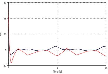
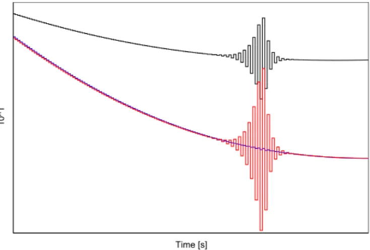
realized phase space. As it can be seen, the trajectories move absolutely together. In Figs 5-8 the desired, reference, and recalculated (by the approximate model) torques are displayed, where the desired and realized torques are almost the same most of the time. First, in Fig 5, everything is shown to be able to approximate the order of it, while, in Fig 6, the previous figure is shown with vertical zoom, so the lines can be seen in more details. In Figs 7 and 8 three examples are given for the adaptive controller loosing its convergensity and slowly gaining it back with a sliding mode kind chattering.
Fig 10 illustrates the decline of A0 from 6. Finally, in Fig 9 the tracking error is shown, it is reduced by one and a half order compared to the nonadaptive case.
V. CONCLUSIONS
Nowadays, control of dynamical systems with uncertainties is a common problem. Many solutions can be found in the literature, one of these methods is the family of Robust Fixed Point Transformations (RFPT) with local basin of attraction, which has very similar properties to Sliding Mode Controllers.
RFPT is based on a function which can locally converge to the ideal solution. In this paper, authors show that though RFPT can loose its local convergensity, it can still improve a simple controller’s results, and this improvement makes the controller’s behavior very similar to that of a sliding mode
Fig. 5. Desired, realized (lower, they are on the same line), and recalculated (by the approximate model; upper) torques, adaptive case
Fig. 6. Desired, realized (lower, they are on the same line), and recalculated (by the approximate model; upper) torques, adaptive case, vertically zoomed
controller. The similarity includes the so called chattering effect, but a simple algorithm is introduced to minimize the fluctuation of the control signal. Simulations show that the non convergent RFPT can reduce the tracking error achieved by a simple PID controller with more than one order.
ACKNOWLEDGMENT
The authors gratefully acknowledge the grant provided by the project T ´AMOP-4.2.2/B-10/1-2010-0020, support of the scientific training, workshops, and establishing talent manage- ment system at ´Obuda University.
REFERENCES
[1] A.M. Lyapunov,A general task about the stability of motion(in Russian), PhD Thesis, 1892
[2] A.M. Lyapunov, Stability of motion, Academic Press, New-York and London, 1966
[3] Tanaka, K., Wang, H.O, Fuzzy Control Systems Design and Analysis.
New York: John Wiley & Sons, Inc., 2001
[4] V´arkonyi-K´oczy, A.R., State Dependant Anytime Control Methodology for Non-linear Systems, International Journal of Advanced Computational Intelligence and Intelligent Informatics (JACIII), Vol. 12, No. 2, pp. 198–
205, March 2008
Fig. 7. Desired (inner, almost one straight line), realized (outer, the biggest chattering), and recalculated (by the approximate model; middle line, medium chattering) torques, adaptive case, in details
Fig. 8. Desired (lower, inner, almost one soft curve), realized (lower, outer, the biggest chattering), and recalculated (by the approximate model; upper, medium chattering) torques, adaptive case, in details
Fig. 9. The decline ofA0
[5] R. Isermann, K.H. Lachmann, and D. Matko,Adaptive Control Systems, Prentice-Hall, New York DC, USA, 1992
[6] Jean-Jacques E. Slotine, W. Li,Applied Nonlinear Control, Prentice Hall International, Inc., Englewood Cliffs, New Jersey 1991
[7] Charles C. Nguyen, Sami S. Antrazi, Zhen-Lei Zhou, Charles E. Campbell Jr.: Adaptive control of a stewart platform-based manipulator, Journal of Robotic Systems, Volume 10, Number 5, 1993, pp. 657–687
[8] R.M. Murray, Z. Li, S.S. Sastry: A mathematical introduction to robotic manipulation, CRC Press, New York, 1994.
[9] R. Kamnik, D. Matko and T. Bajd: Application of Model Reference Adaptive Control to Industrial Robot Impedance Control, Journal of Intelligent and Robotic Systems, vol. 22, pp. 153–163, 1998.
[10] J. Soml´o, B. Lantos, P.T. C´at, Advanced Robot Control, Akad´emiai Kiad´o, Budapest, Hungary, 2002
[11] K. Hosseini–Suny, H. Momeni, and F. Janabi-Sharifi, Model Reference Adaptive Control Design for a Teleoperation System with Output Predic- tion,J Intell Robot Syst, DOI 10.1007/s10846-010-9400-4, pp. 1–21, 2010.
[12] C. Vecchio, Sliding Mode Control: Theoretical developments and applications to uncertain mechanical systems, http://www- 3.unipv.it/dottIEIE/tesi/2008/c vecchio.pdf, 2008
Fig. 10. The tracking error, adaptive case
[13] J.K. Tar, I.J. Rudas, J.F. Bit´o, T.A. V´arkonyi, Chaos Synchronization by Model Reference Adaptive Control Using Fixed Point Transformations, Proc. of the 13thIASTED International Conference on Intelligent Systems and Control (ISC 2011), Cambridge, United Kingdom, pp. 23–28, 2011 [14] T.A.V´arkonyi, J.K. Tar, I.J. Rudas, Fuzzy Parameter Tuning in the
Stabilization of an RFPT-based Adaptive Control for an Underactuated System, Proc. of the 12thInternational Symposium on Computational Intelligence and Informatics (CINTI 2011) , Budapest, Hungary, pp. 63–68, 2011
[15] Banach, S. ”Sur les op´erations dans les ensembles abstraits et leur application aux quations int´egrales.” Fund. Math. 3, pp. 133-181, 1922 [16] B. Van der Pol, Philos. Mag. 7 (3) 65, 1927.
[17] F.M. Moukam, Kakmeni, S. Bowong, C. Tchawoua , E. Kaptouom:
Chaos control and synchronization of aΦ6-Van der Pol oscillator, Physics Letters A , 322, 305- 323, 2004
[18] J. ˇZilkov´a, J. Timko, P. Girovsk´y: Nonlinear System Control Using Neural Networks, Acta Polytechnica Hungarica, 3(4), pp. 85–94, 2006